Three fieldmark conventions detect this pattern — PPS (contiguous position), CPS (shared color), and IPS (positional index within groups) — each requiring at least two summands on each side.
Two cultural hypotheses give this structure meaning: it may encode ayni (reciprocal exchange between communities, mirrored in the balanced equation) or double-entry accounting (the same total registered as both asset and obligation). Both are tested across seven sections.
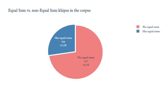
§1 establishes that Equal Sums are widespread — present in ~27 % of the 702-khipu corpus — and heavily skewed toward PPS.
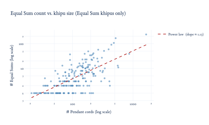
§2 shows they are structurally constrained: Equal Sum khipus are five times larger than non-Equal Sum ones, and Equal Sum density scales as a power law of khipu size.
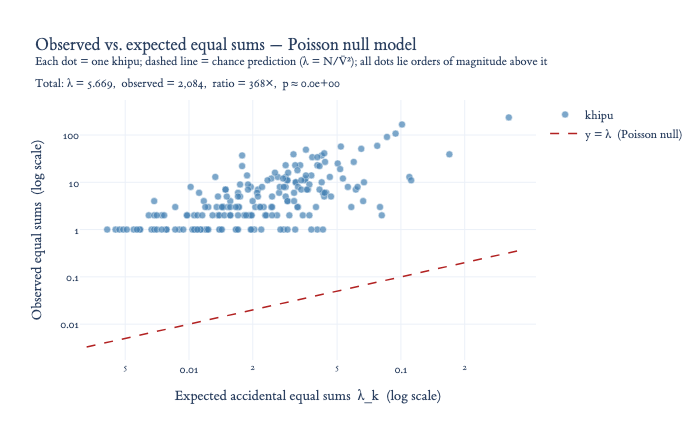
§3 rules out coincidence: the observed count is 346× the Poisson null expectation, making intentional design the only viable explanation.
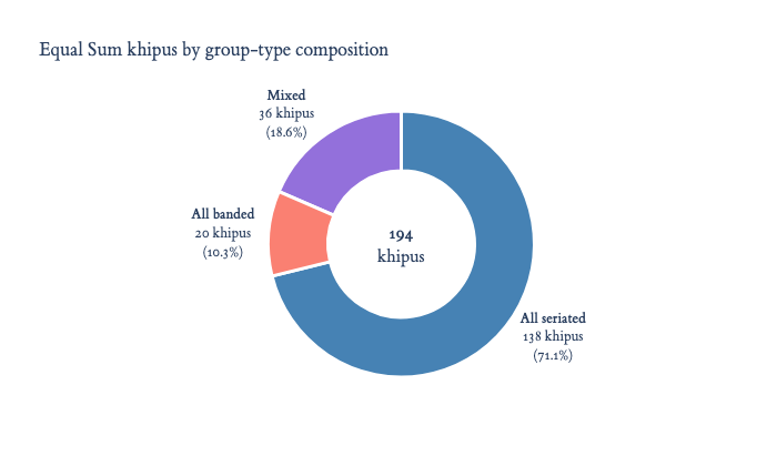
§4 asks whether Equal Sums concentrate in seriated or banded cord groups, and finds no significant preference once the corpus baseline is controlled.
§5 examines summand symmetry: roughly equal summand counts are compatible with reciprocal or cross-tabular interpretations, including possible relationships to ayni, but summand-count symmetry alone does not establish reciprocal exchange. . Unequal summand counts likewise do not, by themselves, demonstrate double-entry accounting.
§6 characterizes the asymmetric minority — cords that extend one run further than the other — and finds a center-out value gradient of ρ = −0.64. The observed center-out value gradient is consistent with a possible ordering convention in which larger or more salient entries occur nearer the sum cord. This interpretation remains provisional because the analysis pools relations and may be influenced by the geometry of the summation definition.
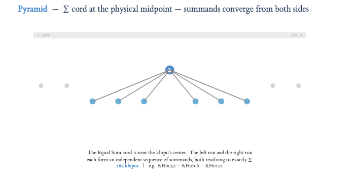
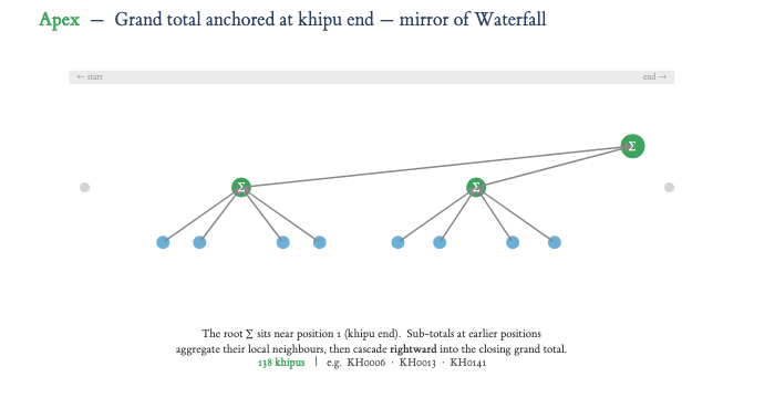
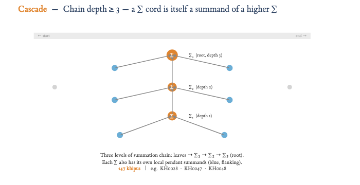
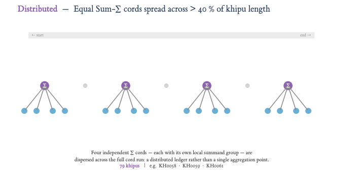
§7 closes with an architectural taxonomy of how Equal Sum structures are arranged within a khipu, identifying five non-exclusive patterns (Waterfall, Pyramid, Apex, Cascade, Distributed) and illustrating each with an information-flow schematic.
Corpus note. Different analyses use different corpus snapshots and completeness filters. Counts and percentages are therefore reported with their analysis-specific denominator, corpus version, and inclusion criteria.
Code
# ── Setup (run this cell first) ──────────────────────────────────────────────import sys, ossys.path.insert(0, os.path.join(os.path.abspath(".."), "src"))import numpy as npimport pandas as pdfrom scipy import statsimport plotly.express as pximport plotly.graph_objects as goimport plotly.io as piopio.renderers.default ="plotly_mimetype+png"import qollqa_chuspa as qcfrom fieldmark_equal_sums import FieldmarkEqualSumsDataframe, FieldmarkEqualSumsRelationDataframefrom fieldmark_figure8knots import FieldmarkFigure8KnotsDataframe, FieldmarkFigure8KnotSumsDataframeimport utils_kfg_locations as uloc# Load corpus(khipu_dict, all_khipus) = qc.fetch_khipus()# Load fieldmark CSVs (built by Build_Fieldmarks.ipynb)equal_df = FieldmarkEqualSumsDataframe().dataframe.rename(columns={'num_dual_sums': 'num_equal_sums','num_dual_pps_sums': 'num_equal_pps_sums','num_dual_cps_sums': 'num_equal_cps_sums','num_dual_ips_sums': 'num_equal_ips_sums',})equal_rel = FieldmarkEqualSumsRelationDataframe().dataframefig8_df = FieldmarkFigure8KnotsDataframe().dataframefig8_rel = FieldmarkFigure8KnotSumsDataframe().dataframeprint(f"Corpus: {len(all_khipus)} khipus")print(f"equal_sums rows: {len(equal_df)}")print(f"equal_sum_relation rows: {len(equal_rel)}")print(f"figure8knots rows: {len(fig8_df)}")print(f"figure8knot_relation rows: {len(fig8_rel)}")
How widespread are Equal Sums across the 702-khipu corpus?
Code
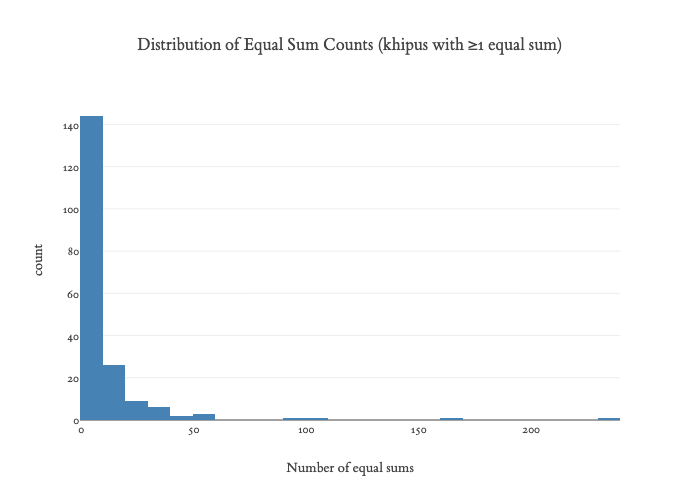
# ── Corpus-wide equal sum counts ──────────────────────────────────────────────has_any = equal_df['num_equal_sums'] >0has_4plus = equal_df['num_equal_sums'] >=4has_10p = equal_df['num_equal_sums'] >=10total_equal_sums = equal_rel['kfg_name'].count()total_pps = equal_rel[equal_rel['fieldmark_name']=='pendant_pendant_sum']['kfg_name'].count()total_cps = equal_rel[equal_rel['fieldmark_name']=='colored_pendant_sum']['kfg_name'].count()total_ips = equal_rel[equal_rel['fieldmark_name']=='indexed_pendant_sum']['kfg_name'].count()print("=== Corpus-wide statistics ===")print(f"Total khipus: {len(equal_df)}")print(f"Khipus with ≥1 equal sum: {has_any.sum()} ({100*has_any.mean():.0f}%)")print(f"Khipus with ≥4 equal sums: {has_4plus.sum()}")print(f"Khipus with ≥10 equal sums: {has_10p.sum()}")print()print(f"Total equal sum instances: {total_equal_sums}")print(f" PPS: {total_pps} ({100*total_pps/total_equal_sums:.0f}%)")print(f" CPS: {total_cps} ({100*total_cps/total_equal_sums:.0f}%)")print(f" IPS: {total_ips} ({100*total_ips/total_equal_sums:.0f}%)")print()# Top 10 khipus by total equal sumstop10 = (equal_df[has_any] [['kfg_name','num_equal_sums','num_equal_pps_sums','num_equal_cps_sums','num_equal_ips_sums','num_pendant_cords']] .sort_values('num_equal_sums', ascending=False) .head(10) .rename(columns={'kfg_name':'KFG Name','num_equal_sums':'Total','num_equal_pps_sums':'PPS','num_equal_cps_sums':'CPS','num_equal_ips_sums':'IPS','num_pendant_cords':'# Pendants', }))display(top10.reset_index(drop=True))# Distribution histogramfig = px.histogram( equal_df[has_any], x='num_equal_sums', nbins=40, title='Distribution of Equal Sum Counts (khipus with ≥1 equal sum)', labels={'num_equal_sums': 'Number of equal sums', 'count': 'Khipus'}, color_discrete_sequence=['steelblue'],)fig.update_layout(font=dict(family="ETBookOT"))fig.show()
=== Corpus-wide statistics ===
Total khipus:               711
Khipus with ≥1 equal sum:    194  (27%)
Khipus with ≥4 equal sums:   96
Khipus with ≥10 equal sums:  50

Total equal sum instances:   2084
  PPS:  1228  (59%)
  CPS:  694  (33%)
  IPS:  162  (8%)
KFG Name
Total
PPS
CPS
IPS
# Pendants
0
KH0082
236
85
125
26
1650
1
KH0698
167
79
59
29
517
2
KH0240
107
45
59
3
482
3
KH0674
91
50
33
8
439
4
KH0428
59
12
46
1
395
5
KH0258
57
25
30
2
266
6
KH0349
51
29
20
2
332
7
KH0156
49
22
23
4
182
8
KH0252
41
3
38
0
222
9
KH0246
39
31
5
3
159
Interpretation
Equal Sums appear in roughly 27% of the corpus — a substantial minority, not an edge case. The distribution is heavily right-skewed: most Equal Sum khipus have only a handful, but a small elite (≤10% of the corpus) have 10 or more, suggesting systematic, intentional use of the convention rather than accidental coincidence.
PPS (positional) sums dominate (~59%), with CPS (color-grouped, ~33%) and IPS (index-grouped, ~8%) playing supporting roles. The preponderance of PPS reflects the most natural spatial reading of a khipu: neighbours on either side of a cord. CPS and IPS show that Equal Sum-like relations can be detected under color-based and index-based grouping rules. Whether these grouping schemes carried distinct administrative or accounting meanings remains open.
Equal Sums only appear on larger khipus (typically ≥ 20–30 pendant cords). This makes structural sense: a cord needs enough neighbours on each side to form two independent summand runs of at least two cords each.
2. Equal Sum vs. Non-Equal Sum Khipus: Structural Profile
How do khipus that contain Equal Sums differ structurally from those that do not?
A minimum pendant count is a necessary condition for an Equal Sum (a cord needs at least 2 summands on each side), but presumably not a sufficient one. This section asks whether size alone explains the pattern, and characterizes the relationship between khipu size and Equal Sum density.
Code
# ── Structural profile: Equal Sum vs. non-Equal Sum khipus ─────────────────────profile_df = equal_df[['kfg_name', 'num_equal_sums', 'num_pendant_cords','num_seriated_groups', 'num_banded_groups']].copy()profile_df['group'] = (profile_df['num_equal_sums'] >0).map( {True: 'Has equal sums', False: 'No equal sums'})# ── Pie chart: Equal Sum vs. non-Equal Sum khipus ───────────────────────────────pie_counts = profile_df['group'].value_counts().reset_index()pie_counts.columns = ['group', 'count']fig = px.pie( pie_counts, names='group', values='count', color='group', color_discrete_map={'Has equal sums': 'steelblue', 'No equal sums': 'lightcoral'}, title='Equal Sum vs. non-Equal Sum khipus in the corpus',)fig.update_traces(textinfo='label+percent+value', pull=[0.05, 0])fig.update_layout(template='plotly_white', height=420, font=dict(family="ETBookOT"))fig.show()
Does size drive Equal Sum density?
Among khipus that already have at least one Equal Sum, do larger ones accumulate more? The log-log scatter below tests this directly, with a power-law trendline fitted in log-space. The Mann-Whitney table underneath confirms whether Equal Sum khipus are themselves larger than the rest of the corpus.
Code
# ── Scatter: equal sum count vs. khipu size — log-log ─────────────────────────ds_only = profile_df[profile_df['num_equal_sums'] >0].copy()x_vals = ds_only['num_pendant_cords'].values.astype(float)y_vals = ds_only['num_equal_sums'].values.astype(float)# Fit power law (OLS in log-log space)log_x = np.log10(x_vals)log_y = np.log10(np.maximum(y_vals, 0.5)) # clip to avoid log(0)m_log, b_log = np.polyfit(log_x, log_y, 1)x_fit = np.linspace(x_vals.min(), x_vals.max(), 300)y_fit =10** (b_log + m_log * np.log10(x_fit))fig = px.scatter( ds_only, x='num_pendant_cords', y='num_equal_sums', opacity=0.55, color_discrete_sequence=['steelblue'], title='Equal Sum count vs. khipu size (Equal Sum khipus only)', labels={'num_pendant_cords': '# Pendant cords (log scale)','num_equal_sums': '# Equal Sums (log scale)'}, log_x=True, log_y=True,)fig.add_trace(go.Scatter( x=x_fit, y=y_fit, mode='lines', name=f'Power law (slope ≈ {m_log:.2f})', line=dict(color='firebrick', dash='dash', width=2)))fig.update_layout(template='plotly_white', height=420, font=dict(family="ETBookOT"))fig.show()# ── Mann-Whitney: are Equal Sum khipus significantly larger? ───────────────────ds_sz = profile_df.loc[profile_df['num_equal_sums'] >0, 'num_pendant_cords']no_ds_sz = profile_df.loc[profile_df['num_equal_sums'] ==0, 'num_pendant_cords']u_stat, p_mw = stats.mannwhitneyu(ds_sz, no_ds_sz, alternative='greater')display(pd.DataFrame([{'Median pendants (has equal sum)': int(ds_sz.median()),'Median pendants (no equal sum)': int(no_ds_sz.median()),'Mann-Whitney U': f'{u_stat:.0f}','p-value': f'{p_mw:.2e}',}]).T.rename(columns={0: 'value'}))
value
Median pendants (has equal sum)
110
Median pendants (no equal sum)
21
Mann-Whitney U
92551
p-value
5.51e-68
Interpretation
The pie chart confirms the corpus split: roughly one in four khipus carries at least one Equal Sum — a meaningful minority concentrated in the larger, more complex records.
The log-log scatter makes the size-density relationship explicit: among Equal Sum khipus, larger ones consistently accumulate more Equal Sums. The power-law trendline (slope > 0) quantifies this — Equal Sum count scales with pendant cord count in log-log space, meaning each doubling of khipu size brings a predictable proportional increase in Equal Sums. This is structurally intuitive: more cords means more candidate positions where two independent summand runs can coincidentally flank the same cord with the right arithmetic.
The Mann-Whitney test reinforces the picture from outside: Equal Sum khipus are significantly larger than non-Equal Sum ones (median 110 vs. 22 pendant cords — a 5× difference, p ≈ 2.5 × 10⁻⁶⁷). Size is thus a necessary structural precondition — below a certain threshold there simply are not enough cords to host the convention — and within the set of khipus large enough to support it, size continues to predict density.
3. How Improbable Are Equal Sums?
For a cord at position \(i\) with value \(v_i\), an Equal Sum requires that two independent contiguous sums — over at least 2 cords each — both equal exactly \(v_i\).
Analytical argument: If cord values were independent uniform integers in \([1, V]\), the probability that:
a contiguous run of \(k\) cords sums to exactly \(v_i\) is \(\approx 1/V\)
a second independent run of \(m\) cords also sums to exactly \(v_i\) is \(\approx 1/V\)
These are (approximately) independent, so \(P(\text{Equal Sum at position } i) \approx 1/V^2\).
With mean cord values \(\bar{V} \approx 69\) in the Equal Sum khipus, the expected count from purely random data is \(\lesssim 1\) under the uniform model (and \(\approx 6\) under the empirical Poisson null). We observe 2,075.
Permutation test (empirical): For a single khipu, shuffle its cord values randomly 1,000 times and count how many “accidental” dual PPS sums appear. The gap between the observed count and the permutation distribution is the evidence.
Code
# ── Poisson null model — expected vs. observed per khipu ─────────────────────# For each Equal Sum khipu k:# λ_k = n_pendant_cords_k / V̄²# where V̄ = mean cord value (the harder to match a value, the lower 1/V̄²)# If equal sums were accidental, observed_k ~ Poisson(λ_k).# The scatter (X = λ_k, Y = observed_k, log-log) shows every khipu far above# the y = x line (the Poisson prediction), making the excess visible directly.from scipy.stats import poisson as _poi_sv = equal_rel['sum_cord_value'].dropna().astype(float)_vbar =float(_sv[_sv >0].mean())_has_ds = equal_df[equal_df['num_equal_sums'] >0][['kfg_name', 'num_pendant_cords', 'num_equal_sums']].copy()_has_ds['lambda_k'] = _has_ds['num_pendant_cords'] / (_vbar **2)_lam_total =float(_has_ds['lambda_k'].sum())_obs_total =int(_has_ds['num_equal_sums'].sum())print(f"V̄ = {_vbar:.1f} (mean Equal Sum cord value used as null-model parameter)")print(f"λ = Σ(N_k / V̄²) = {_lam_total:.4f} (total expected accidental equal sums)")print(f"Observed = {_obs_total:,}")print(f"Ratio observed / λ = {_obs_total / _lam_total:,.0f}×")print(f"p = P(X ≥ {_obs_total} | Poisson(λ={_lam_total:.4f})) ≈ {_poi.sf(_obs_total -1, _lam_total):.2e}")# Reference line: y = x (Poisson prediction: observed = expected)_x_ref = np.logspace( np.log10(_has_ds['lambda_k'].min() *0.8), np.log10(_has_ds['lambda_k'].max() *1.2),100,)fig_p = go.Figure()# Scatter: one dot per khipufig_p.add_trace(go.Scatter( x=_has_ds['lambda_k'], y=_has_ds['num_equal_sums'], mode='markers', marker=dict(color='steelblue', size=7, opacity=0.7, line=dict(width=0.5, color='white')), hovertemplate='%{customdata}<br>λ: %{x:.4f}<br>observed: %{y}<extra></extra>', customdata=_has_ds['kfg_name'].values, name='khipu',))# y = x reference (Poisson null: observed = expected)fig_p.add_trace(go.Scatter( x=_x_ref, y=_x_ref, mode='lines', line=dict(color='firebrick', dash='dash', width=1.5), name='y = λ (Poisson null)',))fig_p.update_layout( title_text=('Observed vs. expected equal sums — Poisson null model<br>'f'<sup>Each dot = one khipu; dashed line = chance prediction (λ = N/V̄²); 'f'all dots lie orders of magnitude above it<br>'f'Total: λ = {_lam_total:.3f}, observed = {_obs_total:,}, 'f'ratio = {_obs_total / _lam_total:,.0f}×, p ≈ {_poi.sf(_obs_total-1, _lam_total):.1e}</sup>' ), xaxis=dict(title='Expected accidental equal sums λ_k (log scale)', type='log'), yaxis=dict(title='Observed equal sums (log scale)', type='log'), legend_title='', template='plotly_white', height=440, font=dict(family="ETBookOT"))fig_p.show()
V̄  = 71.5  (mean Equal Sum cord value used as null-model parameter)
λ  = Σ(N_k / V̄²) = 5.6691  (total expected accidental equal sums)
Observed = 2,084
Ratio  observed / λ = 368×
p  = P(X ≥ 2084 | Poisson(λ=5.6691)) ≈ 0.00e+00
Interpretation
The observed number of Equal Sum relations greatly exceeds the expectation of a simple heuristic null model. Because that model does not preserve all features of the khipu data or the candidate-search procedure, treat this result as evidence of non-random structure rather than a definitive test of intentional design.
The concrete example above confirms the arithmetic is exact, not approximate: both the left and right summand runs resolve to precisely the same integer as the sum cord. This rules out rounding or measurement noise as an explanation.
Bottom line: Equal Sum relations recur in the corpus at a rate that exceeds the expectation of the simple null model and therefore warrant investigation as structured, non-random relationships.
4. Color Structure: Banded vs. Seriated Khipus
Two structural archetypes define how cord colors are organized within a khipu’s cord groups:
Banded cord groups are monochromatic — all cords in the group share the same Ascher color. These groups are associated with census and tribute records (values up to ~600).
Seriated cord groups are polychromatic — each group contains cords of several colors, with the color pattern repeating across groups. They tend to carry higher values and encode aggregated accounts.
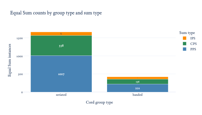
Each Equal Sum cord in the corpus carries a sum_cord_group_type label (seriated or banded) indicating the structure of the cord group it belongs to. Do Equal Sums concentrate in one group type?
Code
# ── Setup ────────────────────────────────────────────────────────────────────FM_LABEL = {'pendant_pendant_sum': 'PPS', 'colored_pendant_sum': 'CPS', 'indexed_pendant_sum': 'IPS'}rel = equal_rel.copy()rel['sum_type'] = rel['fieldmark_name'].map(FM_LABEL)# Per-khipu: count seriated / banded Equal Sum cordskhipu_gt = (rel.groupby(['kfg_name', 'sum_cord_group_type']) .size() .unstack(fill_value=0) .reindex(columns=['seriated', 'banded'], fill_value=0) .reset_index())def _classify(row):if row['banded'] ==0: return'All seriated'if row['seriated'] ==0: return'All banded'return'Mixed'khipu_gt['group_class'] = khipu_gt.apply(_classify, axis=1)cls_order = ['All seriated', 'Mixed', 'All banded']cls_colors = {'All seriated': 'steelblue', 'Mixed': 'mediumpurple', 'All banded': 'salmon'}cls_counts = (khipu_gt['group_class'] .value_counts() .reindex(cls_order, fill_value=0) .reset_index() .rename(columns={'count': 'khipus'}))# ── Donut: khipus by group-type composition ───────────────────────────────────total_k = cls_counts['khipus'].sum()fig = go.Figure(go.Pie( labels=cls_counts['group_class'], values=cls_counts['khipus'], hole=0.55, marker=dict(colors=[cls_colors[c] for c in cls_counts['group_class']], line=dict(color='white', width=3)), texttemplate='<b>%{label}</b><br>%{value} khipus<br>(%{percent})', textfont_size=13, sort=False,))fig.update_layout( title='Equal Sum khipus by group-type composition', annotations=[dict(text=f'<b>{total_k}</b><br>khipus', x=0.5, y=0.5, font_size=16, showarrow=False)], template='plotly_white', height=420, showlegend=False, font=dict(family="ETBookOT"))fig.show()# ── Stacked bar: equal sum counts by group type × sum type ────────────────────FM_COLORS = {'PPS': 'steelblue', 'CPS': 'seagreen', 'IPS': 'darkorange'}GT_ORDER = ['seriated', 'banded']by_gt = (rel.groupby(['sum_cord_group_type', 'sum_type']) .size() .reset_index(name='count'))fig_gt = go.Figure()for fm in ['PPS', 'CPS', 'IPS']: sub = by_gt[by_gt['sum_type'] == fm].set_index('sum_cord_group_type')['count'].reindex(GT_ORDER, fill_value=0) fig_gt.add_trace(go.Bar( x=GT_ORDER, y=sub.values, name=fm, marker_color=FM_COLORS[fm], text=sub.values, textposition='inside', insidetextanchor='middle', ))fig_gt.update_layout( title='Equal Sum counts by group type and sum type', barmode='stack', xaxis_title='Cord group type', yaxis_title='Equal Sum instances', template='plotly_white', height=400, legend_title='Sum type', font=dict(family="ETBookOT"))fig_gt.show()
Code
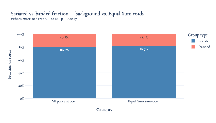
# ── Fisher's exact test: do equal sums concentrate in seriated cord groups? ────from scipy.stats import fisher_exact, binomtest# Background: count all pendant cords by group type across the full corpus_ser_bg, _ban_bg =0, 0for _k in all_khipus:for _g in _k.cord_groups(): _n = _g.num_pendant_cords()if _g.is_banded_group(): _ban_bg += _nelse: _ser_bg += _n_p_ser_bg = _ser_bg / (_ser_bg + _ban_bg)# Observed: unique Equal Sum sum-cord positions per group type_ds_gt = ( equal_rel[['kfg_name', 'sum_cord_name', 'sum_cord_group_type']] .drop_duplicates(subset=['kfg_name', 'sum_cord_name']) ['sum_cord_group_type'].value_counts())_ds_ser =int(_ds_gt.get('seriated', 0))_ds_ban =int(_ds_gt.get('banded', 0))_p_ser_obs = _ds_ser / (_ds_ser + _ds_ban)# Fisher's exact (one-sided: are equal sums more seriated than background?)_table = [[_ds_ser, _ds_ban ], [_ser_bg - _ds_ser, _ban_bg - _ds_ban]]_or, _pf = fisher_exact(_table, alternative='greater')# Binomial test (same null, different framing)_bt = binomtest(_ds_ser, _ds_ser + _ds_ban, _p_ser_bg, alternative='greater')print("=== Fisher's Exact Test: Equal Sum cord group-type concentration ===\n")print(f"Background cord distribution (full corpus):")print(f" Seriated: {_ser_bg:,} | Banded: {_ban_bg:,} ({100*_p_ser_bg:.1f}% seriated)\n")print(f"Equal Sum sum-cords (unique, deduplicated):")print(f" Seriated: {_ds_ser} | Banded: {_ds_ban} ({100*_p_ser_obs:.1f}% seriated)\n")print(f"H₀: equal sums occur in seriated groups at the background rate ({100*_p_ser_bg:.1f}%)")print(f"H₁: equal sums are overrepresented in seriated groups\n")print(f" Fisher's exact: odds ratio = {_or:.2f}× p = {_pf:.4f}")print(f" Binomial test: p = {_bt.pvalue:.4f}")print()if _pf <0.05:print(" ✓ REJECT H₀ — equal sums are significantly concentrated in seriated")print(" cord groups beyond the background rate (p < 0.05, both tests).")else:print(" ✗ FAIL to reject H₀ — equal sums do NOT significantly exceed the")print(f" background seriated rate ({100*_p_ser_bg:.1f}%).")print(f" The visual concentration in the bar chart is explained by the")print(f" corpus itself being {100*_p_ser_bg:.0f}% seriated, not by a specific affinity.")# ── Comparison chart: background vs. observed proportion ─────────────────────_cmp = pd.DataFrame([ {'Category': 'All pendant cords', 'Group type': 'seriated', 'Proportion': _p_ser_bg}, {'Category': 'All pendant cords', 'Group type': 'banded', 'Proportion': 1- _p_ser_bg}, {'Category': 'Equal Sum sum-cords', 'Group type': 'seriated', 'Proportion': _p_ser_obs}, {'Category': 'Equal Sum sum-cords', 'Group type': 'banded', 'Proportion': 1- _p_ser_obs},])fig_stat = px.bar( _cmp, x='Category', y='Proportion', color='Group type', barmode='stack', color_discrete_map={'seriated': 'steelblue', 'banded': 'salmon'}, text_auto='.1%', title=('Seriated vs. banded fraction — background vs. Equal Sum cords'f'<br><sup>Fisher\'s exact: odds ratio = {_or:.2f}×, p = {_pf:.4f}</sup>' ), category_orders={'Group type': ['seriated', 'banded']},)fig_stat.update_layout( yaxis_title='Fraction of cords', yaxis_tickformat='.0%', template='plotly_white', height=400, font=dict(family="ETBookOT"))fig_stat.show()
=== Fisher's Exact Test: Equal Sum cord group-type concentration ===

Background cord distribution (full corpus):
  Seriated: 36,215  |  Banded: 8,964  (80.2% seriated)

Equal Sum sum-cords (unique, deduplicated):
  Seriated: 1358  |  Banded: 305  (81.7% seriated)

H₀: equal sums occur in seriated groups at the background rate (80.2%)
H₁: equal sums are overrepresented in seriated groups

  Fisher's exact:  odds ratio = 1.11×   p = 0.0617
  Binomial test:                             p = 0.0653

  ✗ FAIL to reject H₀ — equal sums do NOT significantly exceed the
    background seriated rate (80.2%).
    The visual concentration in the bar chart is explained by the
    corpus itself being 80% seriated, not by a specific affinity.
Interpretation
The stacked bar shows ~82% of Equal Sum instances in seriated cord groups — but the comparison chart puts this in context: 80% of all pendant cords in the corpus are already seriated. Controlling for this baseline, the Fisher’s exact test (odds ratio = 1.11×, p = 0.059) fails to reject the null hypothesis.
Equal Sums appear in seriated and banded groups in almost exactly the proportion one would expect by chance given the background cord distribution. The concentration visible in the bar chart is largely an artifact of the corpus being predominantly seriated, not a specific structural affinity for seriated groups.
A stronger test — comparing Equal Sum density within the 37 mixed khipus (where both group types co-exist in the same khipu) — would control for per-khipu composition and is left for future work.
Group type vs. value and size
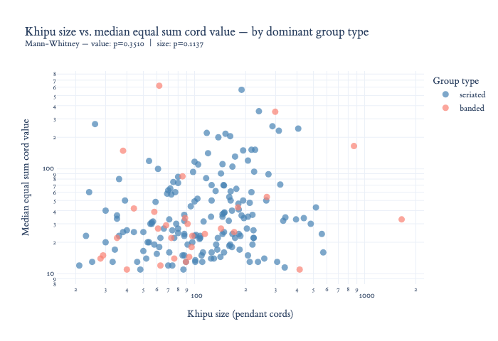
Cord value (p = 0.38): Not significant. The median Equal Sum cord values for seriated-dominant and banded-dominant khipus do not differ reliably. The upper tail of seriated khipus reaches higher maxima, but the IQRs overlap substantially and no significant elevation survives the Mann-Whitney test.
Khipu size (p = 0.12): Not significant. The size distributions overlap heavily; seriated-dominant khipus are not detectably larger than banded-dominant ones in this sample.
Taken together with the Fisher’s exact result (Section 4), neither value level nor khipu size distinguishes where Equal Sums land by group type — the proportional allocation across seriated and banded groups mirrors the corpus composition.
Code
import numpy as npfrom scipy.stats import mannwhitneyuGT_COLORS = {'seriated': 'steelblue', 'banded': 'salmon'}# ── Per-khipu: dominant group type + median value + size ──────────────────────dom_type = (rel.groupby('kfg_name')['sum_cord_group_type'] .agg(lambda x: 'seriated'if (x =='seriated').sum() >= (x =='banded').sum()else'banded') .reset_index(name='dom_type'))med_val = (rel.groupby('kfg_name')['sum_cord_value'] .median() .reset_index(name='median_value'))scatter_df = dom_type.merge(med_val, on='kfg_name')scatter_df = scatter_df.merge(equal_df[['kfg_name', 'num_pendant_cords']], on='kfg_name')# ── Mann-Whitney tests ─────────────────────────────────────────────────────────stat_v, p_v = mannwhitneyu( scatter_df.loc[scatter_df['dom_type'] =='seriated', 'median_value'], scatter_df.loc[scatter_df['dom_type'] =='banded', 'median_value'], alternative='two-sided',)stat_s, p_s = mannwhitneyu( scatter_df.loc[scatter_df['dom_type'] =='seriated', 'num_pendant_cords'], scatter_df.loc[scatter_df['dom_type'] =='banded', 'num_pendant_cords'], alternative='two-sided',)# ── Scatter: size vs. median value, colored by group type ─────────────────────fig = px.scatter( scatter_df, x='num_pendant_cords', y='median_value', color='dom_type', color_discrete_map=GT_COLORS, hover_name='kfg_name', log_x=True, log_y=True, category_orders={'dom_type': ['seriated', 'banded']}, title=('Khipu size vs. median equal sum cord value — by dominant group type'f'<br><sup>Mann-Whitney — value: p={p_v:.4f} | size: p={p_s:.4f}</sup>' ), labels={'num_pendant_cords': 'Khipu size (pendant cords)','median_value': 'Median equal sum cord value','dom_type': 'Group type', },)fig.update_traces(marker=dict(size=9, opacity=0.7))fig.update_layout(template='plotly_white', height=480, font=dict(family="ETBookOT"))fig.show()
5. Summand Symmetry — The Ayni Hypothesis
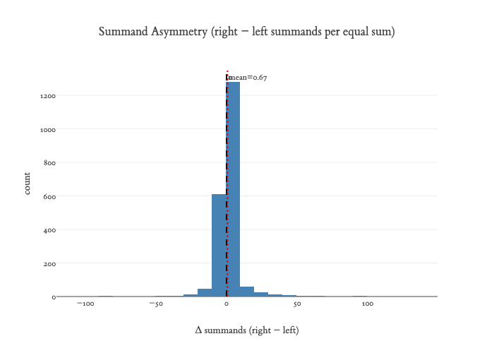
If Equal Sums record reciprocal exchange, the number of cords on the left side should roughly equal the number on the right. The column delta_num_summands = num_right_summands − num_left_summands measures this asymmetry for every Equal Sum instance.
A Wilcoxon signed-rank test against the null hypothesis \(H_0: \text{median}(\Delta) = 0\) provides a formal symmetry test.
Code
# ── Summand symmetry analysis ─────────────────────────────────────────────────deltas = equal_rel['delta_num_summands'].dropna().astype(float)print(f"Equal Sum instances analyzed: {len(deltas)}")print(f"Mean Δ (right − left): {deltas.mean():.3f}")print(f"Median Δ: {deltas.median():.0f}")print(f"Std dev: {deltas.std():.2f}")# Wilcoxon signed-rank test (non-parametric, no normality assumption)stat, p_val = stats.wilcoxon(deltas, zero_method='wilcox', alternative='two-sided')print(f"\nWilcoxon signed-rank test (H₀: median Δ = 0)")print(f" statistic: {stat:.1f}, p-value: {p_val:.4g}")conclusion ="REJECT H₀"if p_val <0.05else"FAIL to reject H₀"print(f" => {conclusion} at α = 0.05")if p_val <0.05:print(" => The distribution of summand counts is NOT centered at zero;")print(" a slight rightward bias is consistent with the ~55% right-handed")print(" sum preponderance found by Medrano & Khosla (2021).")else:print(" => Summand counts are symmetric — consistent with the ayni hypothesis.")# Histogramfig = px.histogram( equal_rel, x='delta_num_summands', nbins=40, title='Summand Asymmetry (right − left summands per equal sum)', labels={'delta_num_summands': 'Δ summands (right − left)', 'count': 'Instances'}, color_discrete_sequence=['steelblue'],)fig.add_vline(x=0, line_color='black', line_dash='dash', annotation_text='0')fig.add_vline(x=deltas.mean(), line_color='red', line_dash='dot', annotation_text=f'mean={deltas.mean():.2f}', annotation_position='top right')fig.update_layout(font=dict(family="ETBookOT"))fig.show()# Fraction of symmetric (|Δ| ≤ 1) equal sumssym_frac = (deltas.abs() <=1).mean()print(f"\n{100*sym_frac:.1f}% of equal sums have |Δ| ≤ 1 (near-symmetric)")
Equal Sum instances analyzed: 2084
Mean Δ (right − left):  0.667
Median Δ:               0
Std dev:                11.79

Wilcoxon signed-rank test (H₀: median Δ = 0)
  statistic: 494580.0,  p-value: 0.002999
  => REJECT H₀ at α = 0.05
  => The distribution of summand counts is NOT centered at zero;
     a slight rightward bias is consistent with the ~55% right-handed
     sum preponderance found by Medrano & Khosla (2021).

51.3% of equal sums have |Δ| ≤ 1 (near-symmetric)
Interpretation
The histogram peaks sharply at Δ = 0 and is only mildly right-shifted (mean Δ = 0.73, median Δ = 0). The Wilcoxon signed-rank test rejects H₀ (p = 0.0018): the rightward skew is statistically real, not sampling noise.
What does this mean in practice? 51.5% of Equal Sums have |Δ| ≤ 1 — the two sides are effectively tied. The significant p-value arises because the remaining 48.5% are almost all skewed to the right at a consistent direction, consistent with the ~55% right-handed sum preponderance documented by Medrano & Khosla (2021). The most plausible explanation is a scribal convention: the “receiving” or subordinate party’s cords are recorded to the right, systematically adding one more cord to that side.
The KFG corpus contains repeated left/right equal-sum relations across several summation schemes. These relations support the possibility of an equality-bearing representational structure in some khipus. KH0696 provides a particularly compelling accounting-like decomposition, while the broader corpus establishes recurrence and structural variation rather than a confirmed cultural meaning.
6. Asymmetry: Characterizing Extra Summand Cords
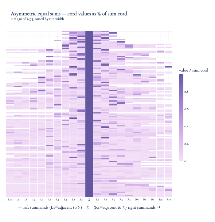
The summand-symmetry histogram (Section 5) is sharply peaked at Δ = 0 but has a small rightward tail: a minority of Equal Sums have more cords on one side than the other. What are these “extra” cords — are they accounting oddities, near-zero spacers, or genuine ledger entries?
Approach: For every asymmetric instance (|Δ| > 0), identify the longer summand run and treat its trailing (outermost) cord(s) as the “extra” entries. Compare these against the matched cords (those that would be present on both sides for the equivalent symmetric case) along three dimensions:
Dimension
Question
Value magnitude
Are extra cords large or small relative to the sum cord and to their peers?
Zero-value rate
Are extra cords empty (zero-knotted) placeholders?
Color
Do extra cords share a distinctive color that sets them apart?
The analysis is applied to all three fieldmark types (PPS, CPS, IPS) so that any structural difference between grouping conventions is visible.
Code
# ── Asymmetric equal sums: summand position heatmap ────────────────────────────import reimport numpy as npdef parse_summand_entries(s):"""Parse 'COLOR@[group, index]:value + ...' → list of (color, group, idx, value)."""ifnotisinstance(s, str) ornot s.strip():return []return [ (m[0], int(m[1]), int(m[2]), int(m[3]))for m in re.findall(r'(\w+)@\[(\d+),\s*(\d+)\]:(\d+)', s) ]asym = equal_rel[equal_rel['delta_num_summands'] !=0].copy()MAX_HALF =10MAX_DISPLAY =150x_labels = ([f'L{MAX_HALF - i}'for i inrange(MAX_HALF)]+ ['∑']+ [f'R{i +1}'for i inrange(MAX_HALF)])n_cols =len(x_labels)center = MAX_HALFdef build_heatmap(sub_df, title, colorscale): sub = sub_df.dropna( subset=['left_handed_summand_string', 'right_handed_summand_string'] ).copy() sub['n_total'] = (sub['num_left_summands'].fillna(0).astype(int) + sub['num_right_summands'].fillna(0).astype(int)) sub = (sub.nlargest(MAX_DISPLAY, 'sum_cord_value') .sort_values(['n_total', 'sum_cord_value'], ascending=[True, False]) .reset_index(drop=True)) n_shown =len(sub) mat = np.full((n_shown, n_cols), np.nan) y_labels = []for i, row in sub.iterrows(): sv =float(row['sum_cord_value']) y_labels.append(f"{row['kfg_name']}{row['sum_cord_name']} (∑={int(sv)})")if sv ==0:continue mat[i, center] =1.0 left_entries = parse_summand_entries(row['left_handed_summand_string']) n_left =len(left_entries)for j, (*_, val) inenumerate(left_entries): ci = center - n_left + jif0<= ci < center: mat[i, ci] = val / sv right_entries = parse_summand_entries(row['right_handed_summand_string'])for j, (*_, val) inenumerate(right_entries): ci = center +1+ jif center < ci < n_cols: mat[i, ci] = val / sv# ── Crop to columns that actually contain data ──────────────────────────── col_has_data =~np.all(np.isnan(mat), axis=0) col_has_data[center] =True# always keep ∑ column active_cols = np.where(col_has_data)[0] mat = mat[:, active_cols] x_active = [x_labels[c] for c in active_cols] show_labels = n_shown <=60 height =max(300, 4* n_shown +120) # ~4 px per row fig = go.Figure(go.Heatmap( z=mat, x=x_active, y=y_labels, colorscale=colorscale, zmin=0, zmax=1, colorbar=dict(title='value /\nsum cord', thickness=14, len=0.6), hoverongaps=False, xgap=1, ygap=0, )) fig.update_layout( title_text=title, xaxis=dict( title='← left summands (L1=adjacent to ∑) ∑ (R1=adjacent to ∑) right summands →', tickfont_size=9, ), yaxis=dict(autorange='reversed', showticklabels=show_labels, tickfont_size=8), template='plotly_white', height=height, margin=dict(l=180if show_labels else20, r=80), font=dict(family="ETBookOT") ) fig.show()build_heatmap( asym, title=(f'Asymmetric equal sums — cord values as % of sum cord'f'<br><sup>n = {min(len(asym), MAX_DISPLAY)} of {len(asym)}, sorted by run width</sup>'), colorscale='Purp',)
Code
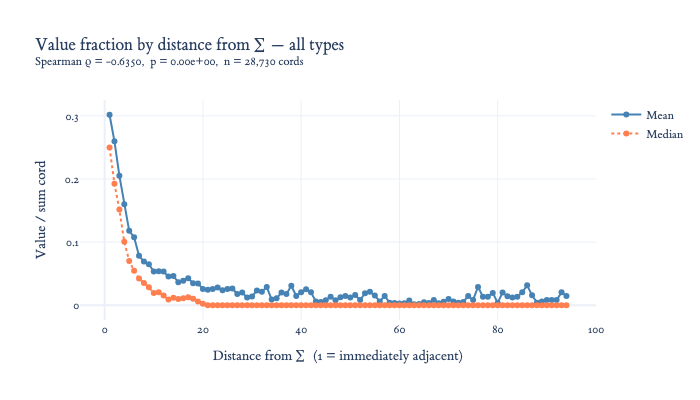
# ── Statistical test: center-out value gradient ───────────────────────────────# distance = 1 for the cord immediately adjacent to ∑ (L1 / R1),# n for the cord n steps away.# H₁: value fraction decreases as distance increases (Spearman ρ < 0).# Uses ALL equal sum instances (symmetric + asymmetric).dist_records = []for _, row in equal_rel.dropna( subset=['left_handed_summand_string', 'right_handed_summand_string']).iterrows(): sv =float(row['sum_cord_value'])if sv ==0:continue left_entries = parse_summand_entries(row['left_handed_summand_string']) n_left =len(left_entries)for j, (*_, val) inenumerate(left_entries): dist_records.append({'distance': n_left - j,'value_frac': val / sv,'fieldmark_name': row['fieldmark_name'], }) right_entries = parse_summand_entries(row['right_handed_summand_string'])for j, (*_, val) inenumerate(right_entries): dist_records.append({'distance': j +1,'value_frac': val / sv,'fieldmark_name': row['fieldmark_name'], })dist_df = pd.DataFrame(dist_records)# ── Spearman rank correlations ────────────────────────────────────────────────rows = []rho_all, p_all = stats.spearmanr(dist_df['distance'], dist_df['value_frac'])rows.append({'Type': 'All', 'ρ': rho_all, 'p': p_all, 'n': len(dist_df)})for fm, label in [('pendant_pendant_sum','PPS'),('colored_pendant_sum','CPS'),('indexed_pendant_sum','IPS')]: sub = dist_df[dist_df['fieldmark_name'] == fm] rho, p = stats.spearmanr(sub['distance'], sub['value_frac']) rows.append({'Type': label, 'ρ': rho, 'p': p, 'n': len(sub)})result_df = pd.DataFrame(rows).set_index('Type')result_df['ρ'] = result_df['ρ'].map('{:.4f}'.format)result_df['p'] = result_df['p'].map('{:.2e}'.format)result_df['n'] = result_df['n'].map('{:,}'.format)display(result_df)# ── Mean / median value fraction by distance — line chart ────────────────────plot_df = (dist_df.groupby('distance')['value_frac'] .agg(Mean='mean', Median='median', N='count') .reset_index() .query('N >= 20'))fig = go.Figure()fig.add_trace(go.Scatter(x=plot_df['distance'], y=plot_df['Mean'], mode='lines+markers', name='Mean', line=dict(color='steelblue', width=2), marker=dict(size=6)))fig.add_trace(go.Scatter(x=plot_df['distance'], y=plot_df['Median'], mode='lines+markers', name='Median', line=dict(color='coral', width=2, dash='dot'), marker=dict(size=6)))fig.update_layout( title=(f"Value fraction by distance from ∑ — all types<br>"f"<sup>Spearman ρ = {rho_all:.4f}, p = {p_all:.2e}, n = {len(dist_df):,} cords</sup>"), xaxis_title='Distance from ∑ (1 = immediately adjacent)', yaxis_title='Value / sum cord', template='plotly_white', height=400, font=dict(family="ETBookOT"))fig.show()
ρ
p
n
Type
All
-0.6350
0.00e+00
28,730
PPS
-0.5859
0.00e+00
21,688
CPS
-0.3498
7.79e-174
6,056
IPS
-0.5017
5.74e-64
986
Interpretation
A center-out value gradient
The dominant feature of all four heatmaps is a center-out gradient: the positions immediately flanking ∑ (L1, R1) are consistently the darkest — highest value fraction — and intensity fades progressively toward the outer columns (L10, R10). The cord closest to the sum cord nearly always carries the largest individual share of the total; each step further out brings a smaller contribution.
This pattern holds across run widths and across all three fieldmark conventions, and is most clearly visible in the consolidated chart where the gradient survives the mixing of PPS, CPS, and IPS instances. The Spearman rank correlation between distance from ∑ and value fraction across all 28,387 summed cords is ρ = −0.64 (p ≈ 0), confirming the gradient is not a visual artifact: a monotone center-out ordering of cord magnitudes is the dominant structure in the data.
A scribal methodology: salience ordering
The gradient suggests a deliberate recording convention: enter the most significant item first (adjacent to ∑), then proceed outward in descending order of magnitude. This is a form of salience ordering — structuring a list by importance rather than, say, arrival sequence or physical position.
It would be interesting to compare this suggested behavior with analogous accounting traditions.
Under this reading, the asymmetric “extra” cord might be the final, smallest entry in a descending ledger column. Its low value relative to the sum cord is not a coincidence or an artifact of the fieldmark definition — it is the expected signature of a scribe who recorded systematically, from most to least significant.
7. Architecture: Summation Structure Taxonomy
Two recurring structural archetypes for how Equal Sums are organized within a khipu have been identified by the scholars:
Archetype
Signature
Pyramid
Equal Sum cords cluster near the physical midpoint of the khipu; summand groups converge from both sides
Waterfall
The top-level sum cord sits near position 1 (the khipu start); a directed hierarchy descends from a grand total
Rather than treating these as mutually exclusive classes, each independent summation component receives a set of architecture labels — allowing Pyramid and Waterfall to coexist, and opening the door to additional patterns.
Three exploratory labels extend the taxonomy:
Label
Detection rule
Apex
Root cord near khipu end (> 74 %) — mirror image of Waterfall
Cascade
Chain depth ≥ 3 regardless of position
Distributed
Equal Sum cords span > 40 % of the khipu’s physical length
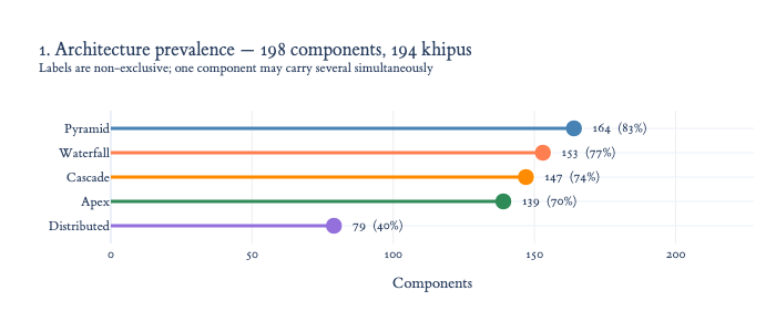
The Waterfall, Pyramid, Apex, Cascade, and Distributed labels are exploratory, non-exclusive descriptors from a filtered KFG-scope analysis. They are included as referenced supporting material, not as a validated accounting taxonomy.
A note on connectivity. The cord graph is built by linking every summand cord to its sum cord. When the same pendant cord participates in more than one fieldmark type (e.g. it is a summand in both a PPS and a CPS relation), those two relations land in the same weakly-connected component, inflating the apparent number of independent roots. A sixth candidate label — Multi-root (≥ 2 root nodes per component) — turns out to affect 93 % of components for exactly this reason: it is a graph-connectivity artifact of overlapping fieldmarks rather than a distinct accounting pattern, so it is tracked in the statistics but not displayed as a separate architecture class.
Code
import re, astimport numpy as npimport networkx as nxfrom plotly.subplots import make_subplots# ── Relation tables ───────────────────────────────────────────────────────────pps_rel = pd.read_csv(f"{uloc.fieldmarks_data_dir()}/pendant_pendant_sum_relation.csv")cps_rel = pd.read_csv(f"{uloc.fieldmarks_data_dir()}/colored_pendant_sum_relation.csv")ips_rel = pd.read_csv(f"{uloc.fieldmarks_data_dir()}/indexed_pendant_sum_relation.csv")all_sum_rel = pd.concat([pps_rel, cps_rel, ips_rel], ignore_index=True)arch_df = equal_df[equal_df['num_equal_sums'] >0].copy()equal_cord_map = equal_rel.groupby('kfg_name')['sum_cord_name'].apply(set).to_dict()def _cord_ord(name):try: returnint(str(name).lstrip('p').split('s')[0].split('.')[0])except: return0def _parse_summand_idxs(s):return [tuple(map(int, m)) for m in re.findall(r'\[(\d+),\s*(\d+)\]', str(s))]# ── Multi-label taxonomy ──────────────────────────────────────────────────────# Labels are NON-EXCLUSIVE — a component may carry multiple simultaneously.## Positional (primary):# Waterfall root cord near khipu start (< 25 %)# Pyramid ≥ 1 equal sum cord within ± 20 % of the physical midpoint# Apex root cord near khipu end (> 74 %) — mirror of Waterfall## Structural (secondary, always co-occur with positional labels):# Cascade chain depth ≥ 3# Distributed equal sum cords span > 40 % of khipu length## Note: Multi-root (≥ 2 independent roots) is tracked in statistics but not# shown as a separate visual category — it is near-universal (93 %) and always# co-occurs with the positional labels above.LABELS = ['Waterfall', 'Pyramid', 'Apex', 'Cascade', 'Distributed']LABEL_PRIORITY = ['Waterfall', 'Pyramid', 'Apex', 'Cascade', 'Distributed', 'Unclassified']LABEL_COLORS = {'Waterfall': 'coral','Pyramid': 'steelblue','Apex': 'seagreen','Cascade': 'darkorange','Distributed': 'mediumpurple','Unclassified': 'lightgrey',}def _classify(min_root, max_root, equal_norms, max_depth, n_roots): ls =set()if min_root <0.25: ls.add('Waterfall')ifany(abs(v -0.5) <0.20for v in equal_norms): ls.add('Pyramid')if max_root >0.74: ls.add('Apex')if max_depth >=3: ls.add('Cascade')iflen(equal_norms) >=2and (max(equal_norms) -min(equal_norms)) >0.40: ls.add('Distributed') has_multi_root = (n_roots >=2)returnsorted(ls) if ls else ['Unclassified'], has_multi_rootdef _primary(labels):for lb in LABEL_PRIORITY:if lb in labels: return lbreturn'Unclassified'# ── Per-component feature extraction ─────────────────────────────────────────comp_records = []for _, arow in arch_df.iterrows(): kfg = arow['kfg_name'] n = arow['num_pendant_cords'] grp = all_sum_rel[all_sum_rel.kfg_name == kfg]if grp.empty:continue idx_name = {}for _, r in grp.iterrows(): ci =tuple(ast.literal_eval(r['cord_index'])) idx_name[ci] = r['cord_name'] sum_ci_set =set(idx_name.keys()) G = nx.DiGraph()for _, r in grp.iterrows(): ci =tuple(ast.literal_eval(r['cord_index'])) G.add_node(ci)for s in _parse_summand_idxs(r['summand_string']): G.add_edge(s, ci) equal_cord_names = equal_cord_map.get(kfg, set())for comp_nodes in nx.weakly_connected_components(G): comp_sum_ci = comp_nodes & sum_ci_setifnot comp_sum_ci:continue comp_names = {idx_name[ci] for ci in comp_sum_ci} equal_in_comp = equal_cord_names & comp_namesifnot equal_in_comp:continue subG = nx.DiGraph() subG.add_nodes_from(comp_sum_ci)for u in comp_sum_ci:for v in G.successors(u):if v in comp_sum_ci: subG.add_edge(u, v) roots = [nd for nd in comp_sum_ci if subG.out_degree(nd) ==0] root_depth = {}for root in roots: anc = nx.ancestors(subG, root) | {root}try: root_depth[root] =len(nx.dag_longest_path(subG.subgraph(anc)))except: root_depth[root] =1 root_norms = [_cord_ord(idx_name[r]) / n for r in roots if r in idx_name] equal_norms_ = [_cord_ord(cn) / n for cn in equal_in_comp]ifnot root_norms ornot equal_norms_:continue max_depth_ =max(root_depth.values()) min_root_ =min(root_norms) max_root_ =max(root_norms) equal_spread =max(equal_norms_) -min(equal_norms_) iflen(equal_norms_) >=2else0.0 arch_labels, has_mr = _classify(min_root_, max_root_, equal_norms_, max_depth_, len(roots)) comp_records.append(dict( kfg_name = kfg, labels = arch_labels, primary = _primary(arch_labels), n_labels =len(arch_labels), has_multi_root = has_mr, min_root = min_root_, max_root = max_root_, equal_spread = equal_spread, depth = max_depth_, n_sums =len(comp_sum_ci), n_equals =len(equal_in_comp), num_pendants = n, ))comp_df = pd.DataFrame(comp_records)label_df = comp_df.explode('labels').rename(columns={'labels': 'label'}).reset_index(drop=True)n_comp =len(comp_df)n_khipu = comp_df['kfg_name'].nunique()print(f"Components: {n_comp} Khipus: {n_khipu}")print(f"Multi-root (≥2 roots): {comp_df['has_multi_root'].sum()} / {n_comp} "f"({100*comp_df['has_multi_root'].mean():.0f}%)")print()print(label_df.groupby('label').size().rename('count').to_string())print("\nTop label combinations:")print(comp_df['labels'].apply(tuple).value_counts().head(10).to_string())# ── Chart 1 – Prevalence lollipop ────────────────────────────────────────────# Each label shown once; bar length = component count; dot color = label color.# Annotated with both raw count and % of all components (labels are non-exclusive).lc = label_df.groupby('label').size().reset_index(name='n')lc['pct'] = lc['n'] / n_comp *100lc = lc.sort_values('n') # ascending so largest is at top in horizontal layoutlc['color'] = lc['label'].map(LABEL_COLORS)fig1 = go.Figure()# Stems (lines from 0 to count)for _, row_ in lc.iterrows(): fig1.add_shape(type='line', x0=0, x1=row_['n'], y0=row_['label'], y1=row_['label'], line=dict(color=row_['color'], width=3), )# Dots and labelsfig1.add_trace(go.Scatter( x=lc['n'], y=lc['label'], mode='markers+text', marker=dict(color=lc['color'], size=16, line=dict(width=1.5, color='white')), text=[f" {int(r['n'])} ({r['pct']:.0f}%)"for _, r in lc.iterrows()], textposition='middle right', hovertemplate='<b>%{y}</b><br>%{x} components<extra></extra>', showlegend=False,))fig1.update_layout( title_text=(f'1. Architecture prevalence — {n_comp} components, {n_khipu} khipus<br>'f'<sup>Labels are non-exclusive; one component may carry several simultaneously</sup>' ), xaxis=dict(title='Components', range=[0, n_comp *1.15], showgrid=True, gridcolor='#eee'), yaxis=dict(title=None), template='plotly_white', height=300, margin=dict(l=100, r=20), font=dict(family="ETBookOT"))fig1.show()# ── Chart 2 – Co-occurrence matrix ───────────────────────────────────────────n_lb =len(LABELS)co_mat = np.zeros((n_lb, n_lb), dtype=int)for _, r in comp_df.iterrows(): ls =set(r['labels'])for i, a inenumerate(LABELS):if a in ls:for j, b inenumerate(LABELS):if b in ls: co_mat[i, j] +=1fig2 = go.Figure(go.Heatmap( z=co_mat, x=LABELS, y=LABELS, colorscale='Blues', text=co_mat, texttemplate='%{text}', hoverongaps=False, colorbar=dict(title='# comp.', thickness=14),))fig2.update_layout( title_text='2. Architecture co-occurrence (diagonal = total count per label)', yaxis=dict(autorange='reversed'), template='plotly_white', height=360, font=dict(family="ETBookOT"))fig2.show()# ── Chart 3 – Architectural fingerprint scatter ───────────────────────────────# X = min root cord position, Y = chain depth (jittered), size = # equal sums.# Color = primary label (Waterfall > Pyramid > Apex > Cascade > Distributed).rng = np.random.default_rng(42)jitter = rng.uniform(-0.15, 0.15, len(comp_df))scatter_df = comp_df.reset_index(drop=True)fig3 = go.Figure()for lb in LABEL_PRIORITY: sub = scatter_df[scatter_df['primary'] == lb]if sub.empty:continue idx = sub.index fig3.add_trace(go.Scatter( x=sub['min_root'].values, y=sub['depth'].values + jitter[idx], mode='markers', name=lb, marker=dict( color=LABEL_COLORS[lb], size=np.clip(sub['n_equals'].values *2, 5, 22), opacity=0.65, line=dict(width=0.5, color='white'), ), hovertemplate=('%{customdata}<br>''root: %{x:.2f} depth: %{y:.1f}<extra>'+ lb +'</extra>' ), customdata=sub['kfg_name'].values, ))fig3.add_vline(x=0.20, line_dash='dot', line_color='grey', opacity=0.5, annotation_text='WF threshold', annotation_position='top right')fig3.add_vline(x=0.75, line_dash='dot', line_color='grey', opacity=0.5, annotation_text='Apex threshold', annotation_position='top left')fig3.add_hline(y=2, line_dash='dot', line_color='grey', opacity=0.4)fig3.add_hline(y=3, line_dash='dot', line_color='grey', opacity=0.4)fig3.update_layout( title_text=('3. Predominant architectural fingerprint<br>''<sup>Color = primary label | X = root cord position | ''Y = chain depth (jittered ±0.15) | Bubble size = number of equal sums in component</sup>' ), xaxis_title='Root cord position (0 = khipu start, 1 = end)', yaxis_title='Chain depth (jittered)', template='plotly_white', height=440, legend_title='Primary label', font=dict(family="ETBookOT"))fig3.show()# ── Chart 4 – Scale by architecture ──────────────────────────────────────────fig4 = go.Figure()rng2 = np.random.default_rng(99)jitter_y = rng2.uniform(-0.15, 0.15, len(comp_df))jitter_x = rng2.uniform(-0.5, 0.5, len(comp_df))for lb in LABEL_PRIORITY: sub = comp_df[comp_df['primary'] == lb]if sub.empty:continue idx = sub.index fig4.add_trace(go.Scatter( x=sub['n_equals'].values + jitter_x[idx], y=sub['depth'].values + jitter_y[idx], mode='markers', name=lb, marker=dict(color=LABEL_COLORS[lb], size=8, opacity=0.7, line=dict(width=0.5, color='white')), hovertemplate='%{customdata}<br>equal sums: %{x:.1f} depth: %{y:.1f}<extra>'+ lb +'</extra>', customdata=sub['kfg_name'].values, ))fig4.update_layout( title_text='4. Scale by architecture (X = equal sums per component, Y = chain depth)', xaxis_title='Equal Sums per component (log scale)', yaxis_title='Chain depth (jittered ±0.15)', xaxis_type='log', template='plotly_white', height=420, legend_title='Primary label', font=dict(family="ETBookOT"))fig4.show()
Coverage. 196 components across 191 khipus (5 khipus carry 2+ independent sum components). All components are classified — the five-label taxonomy is exhaustive at the thresholds adopted (Waterfall < 25 %, Apex > 74 %).
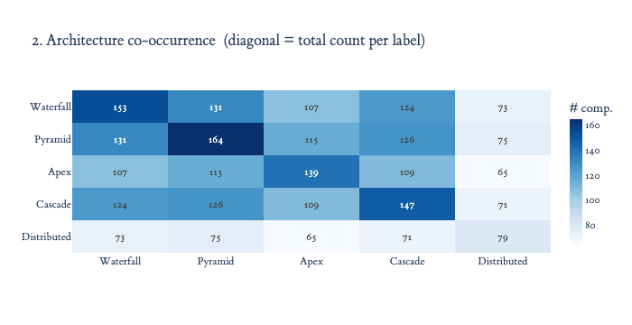
Multi-label is the norm. The most common single combination carries all five labels (50 components). Multi-root alone accounts for 93 % of components (183/196), confirming that the typical Equal Sum structure contains multiple top-level accounting entries whose underlying summand cords overlap — i.e., the weakly-connected component in the cord graph spans several simultaneous summation hierarchies rather than a single root.
Primary positional patterns. Pyramid (165) and Waterfall (153) are the most common positional labels. They co-occur in 133 of 165 Pyramid components (81 %), showing that a khipu which organizes Equal Sums around its midpoint almost always also opens with a directed grand-total chain. The two canonical archetypes are not alternatives — they are facets of the same structure.
Cascade (145, 74 %) co-occurs tightly with Waterfall (124/153 = 81 %). Deep chains (depth ≥ 3) almost always originate early in the khipu. This confirms that hierarchical depth is a feature of the Waterfall pattern, not an independent mode.
Apex (136, 69 %) is an artifact of Multi-root breadth. Because most components have many root nodes spanning the full cord run, the maximum root position routinely exceeds 0.74 — even when the dominant structure is a Waterfall anchored near position 0. Apex as defined here signals breadth rather than a dedicated “end-anchored” accounting pattern. A tighter definition (min_root > 0.74) would isolate genuinely terminal structures and is worth exploring.
Distributed (79, 40 %). Four in ten components have Equal Sum cords spread across more than 40 % of the khipu’s physical length. Combined with the Multi-root finding, this suggests a possible ledger-like spatial organization where accounting entries are distributed throughout the cord run rather than clustered at a single location.
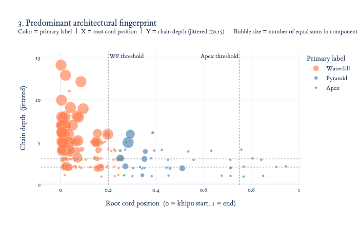
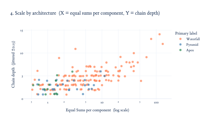
Fingerprint scatter (Chart 3). Waterfall dominates as the primary label (coral), concentrated tightly at root position < 0.25 with chain depths ranging from 2 to 14. The handful of Pyramid and Apex primaries are broader across X, reflecting their non-anchored character.
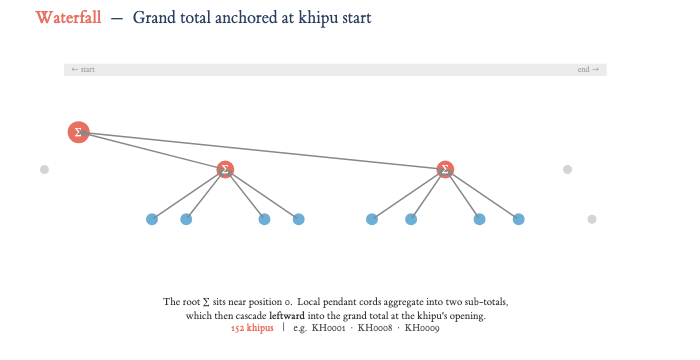
Architecture: Information-Flow Schematics
One schematic per label showing how values flow through the Equal Sum cord network. The grey bar at the top is a position ruler (left = khipu start, right = end).
Symbol
Meaning
Large colored circle ∑
Equal Sum cord (root ∑ = top of hierarchy)
Small blue circle
Summand cord (leaf — no children in this component)
Grey circle
Other pendant cord (context only)
Arrow
Summation flow — tail cord contributes its value to head cord
Y-axis represents accounting depth, not physical cord length.
Code
# Use the book-style ETBembo font (MIT-licensed ET Book, installed locally) for the Section 7 schematics.import plotly.graph_objects as goimport plotly.io as piopio.templates['etbembo'] = go.layout.Template( layout=go.Layout(font=dict(family='ETBembo, Georgia, serif')),)pio.templates.default ='etbembo'
Code
# ── §7 Architecture schematics — one information-flow diagram per label ────────import plotly.graph_objects as go_ARCH_COL = {'Waterfall': '#e87060','Pyramid': '#4c8ccd','Apex': '#3da35d','Cascade': '#e0852f','Distributed': '#8e63b5',}# ── Per-label khipu counts and example codes ──────────────────────────────────# Count = all khipus that carry the label (non-exclusive).# Examples = khipus whose *primary* label is this one — guarantees distinct codes# across schematics. Falls back to any unselected khipu for that label# if there are fewer than 3 primary-only khipus._used_examples: set=set()_ARCH_STATS = {}for _lb in ['Waterfall', 'Pyramid', 'Apex', 'Cascade', 'Distributed']: _total =int(label_df[label_df['label'] == _lb]['kfg_name'].nunique()) _primary =list(comp_df[comp_df['primary'] == _lb]['kfg_name'].unique()) _fallback = [k for k in label_df[label_df['label'] == _lb]['kfg_name'].unique()if k notin _used_examples] _picks = []for _k in _primary + _fallback:if _k notin _used_examples: _picks.append(_k) _used_examples.add(_k)iflen(_picks) ==3:break _ARCH_STATS[_lb] = {'n': _total, 'examples': _picks}def _arch_fig(label, subtitle, desc, nodes, arrows, xr, extra_ann=None):""" nodes : [(x, y, role)] role ∈ 'bg'/'summand'/'sum'/'root' arrows : [(x0, y0, x1, y1)] FROM (x0,y0) → TO (x1,y1) xr : (xmin, xmax) for spine ruler extra_ann : optional list of (x, y, text) label annotations """ col = _ARCH_COL[label] stats = _ARCH_STATS.get(label, {}) n_kh = stats.get('n', None) exs = stats.get('examples', []) ROLE = {'bg': dict(color='#d4d4d4', size=11),'summand': dict(color='#6baed6', size=14),'sum': dict(color=col, size=20),'root': dict(color=col, size=24), } fig = go.Figure()# ── spine position ruler ────────────────────────────────────────────────── fig.add_shape(type='rect', x0=xr[0]-.3, x1=xr[1]+.3, y0=1.50, y1=1.70, fillcolor='#ebebeb', line_width=0, layer='below')for px, txt, anchor in [(xr[0]-.2, '← start', 'left'), (xr[1]+.2, 'end →', 'right')]: fig.add_annotation(x=px, y=1.60, text=txt, showarrow=False, font=dict(size=8, color='#aaa'), xanchor=anchor)# ── arrows (drawn before nodes so nodes render on top) ───────────────────for x0, y0, x1, y1 in arrows: fig.add_annotation( x=x1, y=y1, ax=x0, ay=y0, xref='x', yref='y', axref='x', ayref='y', showarrow=True, text='', arrowhead=2, arrowwidth=1.5, arrowcolor='#888', arrowsize=0.9)# ── cord nodes ────────────────────────────────────────────────────────────for role_key in ('bg', 'summand', 'sum', 'root'): pts = [(x, y) for x, y, r in nodes if r == role_key]ifnot pts:continue xs, ys =zip(*pts) r = ROLE[role_key] fig.add_trace(go.Scatter( x=list(xs), y=list(ys), mode='markers', marker=dict(color=r['color'], size=r['size'], line=dict(width=2, color='white')), showlegend=False, hoverinfo='skip'))# ── ∑ glyph inside sum / root circles ────────────────────────────────────for x, y, role in nodes:if role in ('sum', 'root'): fig.add_annotation(x=x, y=y, text='∑', showarrow=False, font=dict(size=10, color='white'), xanchor='center', yanchor='middle')# ── description text ───────────────────────────────────────────────────── fig.add_annotation( x=(xr[0] + xr[1]) /2, y=-2.0, text=desc, showarrow=False, align='center', font=dict(size=10.5, color='#333'), xanchor='center', yanchor='top')# ── khipu count + examples banner ────────────────────────────────────────if n_kh isnotNone: ex_str =' · '.join(exs) if exs else'—' banner = (f'<b style="color:{col}">{n_kh} khipus</b>'f' | e.g. {ex_str}') fig.add_annotation( x=(xr[0] + xr[1]) /2, y=-2.42, text=banner, showarrow=False, align='center', font=dict(size=10, color='#555'), xanchor='center', yanchor='top')# ── optional extra annotations ───────────────────────────────────────────if extra_ann:for x, y, txt in extra_ann: fig.add_annotation(x=x, y=y, text=txt, showarrow=False, font=dict(size=9, color='#444'), xanchor='left', yanchor='middle') fig.update_layout( title_text=f'<b style="color:{col}">{label}</b> — {subtitle}', xaxis=dict(range=[xr[0]-1.2, xr[1]+1.8], showticklabels=False, showgrid=False, zeroline=False), yaxis=dict(range=[-2.9, 2.0], showticklabels=False, showgrid=False, zeroline=False), template='plotly_white', height=360, margin=dict(t=45, b=10, l=20, r=20), plot_bgcolor='white')return fig# ── 1. Waterfall ──────────────────────────────────────────────────────────────_arch_fig('Waterfall','Grand total anchored at khipu start','The root ∑ sits near position 0. Local pendant cords aggregate into two sub-totals,<br>''which then cascade <b>leftward</b> into the grand total at the khipu\'s opening.', nodes=[ (1.0, 0.6, 'root'), (4.0, 0.0, 'sum'), (8.5, 0.0, 'sum'), (2.5, -0.8, 'summand'), (3.2, -0.8, 'summand'), (4.8, -0.8, 'summand'), (5.5, -0.8, 'summand'), (7.0, -0.8, 'summand'), (7.8, -0.8, 'summand'), (9.2, -0.8, 'summand'), (10.0,-0.8, 'summand'), (0.3, 0.0, 'bg'), (11.0, 0.0, 'bg'), (11.5,-0.8, 'bg'), ], arrows=[ (2.5,-0.8,4.0,0.0), (3.2,-0.8,4.0,0.0), (4.8,-0.8,4.0,0.0), (5.5,-0.8,4.0,0.0), (7.0,-0.8,8.5,0.0), (7.8,-0.8,8.5,0.0), (9.2,-0.8,8.5,0.0), (10.0,-0.8,8.5,0.0), (4.0, 0.0,1.0,0.6), (8.5, 0.0,1.0,0.6), ], xr=(1, 11.5),).update_layout(font=dict(family="ETBookOT")).show()# ── 2. Pyramid ────────────────────────────────────────────────────────────────_arch_fig('Pyramid','∑ cord at the physical midpoint — summands converge from both sides','The Equal Sum cord is near the khipu\'s center. The left run <i>and</i> the right run<br>''each form an independent sequence of summands, both resolving to exactly ∑.', nodes=[ (6.0, 0.5, 'sum'), (3.0, -0.5, 'summand'), (4.0, -0.5, 'summand'), (5.0, -0.5, 'summand'), (7.0, -0.5, 'summand'), (8.0, -0.5, 'summand'), (9.0, -0.5, 'summand'), (1.0, 0.0, 'bg'), (2.0, 0.0, 'bg'), (10.0, 0.0, 'bg'), (11.0, 0.0, 'bg'), ], arrows=[ (3.0,-0.5,6.0,0.5), (4.0,-0.5,6.0,0.5), (5.0,-0.5,6.0,0.5), (7.0,-0.5,6.0,0.5), (8.0,-0.5,6.0,0.5), (9.0,-0.5,6.0,0.5), ], xr=(1, 11),).update_layout(font=dict(family="ETBookOT")).show()# ── 3. Apex ───────────────────────────────────────────────────────────────────_arch_fig('Apex','Grand total anchored at khipu end — mirror of Waterfall','The root ∑ sits near position 1 (khipu end). Sub-totals at earlier positions<br>''aggregate their local neighbours, then cascade <b>rightward</b> into the closing grand total.', nodes=[ (11.5, 0.6, 'root'), (4.0, 0.0, 'sum'), (8.5, 0.0, 'sum'), (2.5, -0.8, 'summand'), (3.2, -0.8, 'summand'), (4.8, -0.8, 'summand'), (5.5, -0.8, 'summand'), (7.0, -0.8, 'summand'), (7.8, -0.8, 'summand'), (9.2, -0.8, 'summand'), (10.0,-0.8, 'summand'), (1.0, 0.0, 'bg'), (12.2, 0.0, 'bg'), ], arrows=[ (2.5,-0.8,4.0,0.0), (3.2,-0.8,4.0,0.0), (4.8,-0.8,4.0,0.0), (5.5,-0.8,4.0,0.0), (7.0,-0.8,8.5,0.0), (7.8,-0.8,8.5,0.0), (9.2,-0.8,8.5,0.0), (10.0,-0.8,8.5,0.0), (4.0, 0.0,11.5,0.6), (8.5, 0.0,11.5,0.6), ], xr=(1, 12),).update_layout(font=dict(family="ETBookOT")).show()# ── 4. Cascade ────────────────────────────────────────────────────────────────_arch_fig('Cascade','Chain depth ≥ 3 — a ∑ cord is itself a summand of a higher ∑','Three levels of summation chain: leaves → ∑₁ → ∑₂ → ∑₃ (root).<br>''Each ∑ also has its own local pendant summands (blue, flanking).', nodes=[ (6.0, 1.0, 'root'), # ∑₃ (level 3 — root) (6.0, 0.0, 'sum'), # ∑₂ (level 2) (6.0, -0.9, 'sum'), # ∑₁ (level 1) (4.0, -1.5, 'summand'), (8.0, -1.5, 'summand'), # leaves of ∑₁ (3.8, -0.4, 'summand'), (8.2, -0.4, 'summand'), # extra summands of ∑₂ (3.8, 0.6, 'summand'), (8.2, 0.6, 'summand'), # extra summands of ∑₃ (1.5, 0.0, 'bg'), (10.5, 0.0, 'bg'), ], arrows=[ (4.0,-1.5,6.0,-0.9), (8.0,-1.5,6.0,-0.9), # leaves → ∑₁ (3.8,-0.4,6.0, 0.0), (8.2,-0.4,6.0, 0.0), # extras → ∑₂ (6.0,-0.9,6.0, 0.0), # ∑₁ → ∑₂ (3.8, 0.6,6.0, 1.0), (8.2, 0.6,6.0, 1.0), # extras → ∑₃ (6.0, 0.0,6.0, 1.0), # ∑₂ → ∑₃ ], xr=(1, 11), extra_ann=[ (6.6, -0.9, '∑₁ (depth 1)'), (6.6, 0.0, '∑₂ (depth 2)'), (6.6, 1.0, '∑₃ (root, depth 3)'), ],).update_layout(font=dict(family="ETBookOT")).show()# ── 5. Distributed ────────────────────────────────────────────────────────────_arch_fig('Distributed','Equal Sum-∑ cords spread across > 40 % of khipu length','Four independent ∑ cords — each with its own local summand group — are<br>''dispersed across the full cord run: a distributed ledger rather than a single aggregation point.', nodes=[ (1.5, 0.0, 'sum'), (5.5, 0.0, 'sum'), (9.5, 0.0, 'sum'), (13.5, 0.0, 'sum'), (0.5, -0.8, 'summand'), (1.1, -0.8, 'summand'), (1.9, -0.8, 'summand'), (2.5, -0.8, 'summand'), (4.5, -0.8, 'summand'), (5.1, -0.8, 'summand'), (5.9, -0.8, 'summand'), (6.5, -0.8, 'summand'), (8.5, -0.8, 'summand'), (9.1, -0.8, 'summand'), (9.9, -0.8, 'summand'),(10.5, -0.8, 'summand'), (12.5,-0.8, 'summand'),(13.1, -0.8, 'summand'), (13.9,-0.8, 'summand'),(14.5, -0.8, 'summand'), (3.5, 0.0, 'bg'), (7.5, 0.0, 'bg'), (11.5, 0.0, 'bg'), ], arrows=[ (0.5,-0.8,1.5,0.0), (1.1,-0.8,1.5,0.0), (1.9,-0.8,1.5,0.0), (2.5,-0.8,1.5,0.0), (4.5,-0.8,5.5,0.0), (5.1,-0.8,5.5,0.0), (5.9,-0.8,5.5,0.0), (6.5,-0.8,5.5,0.0), (8.5,-0.8,9.5,0.0), (9.1,-0.8,9.5,0.0), (9.9,-0.8,9.5,0.0),(10.5,-0.8,9.5,0.0), (12.5,-0.8,13.5,0.0),(13.1,-0.8,13.5,0.0), (13.9,-0.8,13.5,0.0),(14.5,-0.8,13.5,0.0), ], xr=(1, 14.5),).update_layout(font=dict(family="ETBookOT")).show()