Khipu Data Visualization

1.0 Khipu Data Visualization

1.1 Requirements

It’s difficult to understand a khipu from tables. A rendering is necessary. To render khipu adequately, there’s a list of must-haves and nice-to-haves.

Must Haves:

1. Knots must be rendered correctly, including single knots (with the appropriate S/Z/Unknwn slash), long knots, figure-8 knots, etc
2. Cords need to have their cord colors appropriately rendered including solid colors, barber-poles, mottled, striped, etc.
3. Cords need to show their bias/ply (ie. S/Z) and their attachment type (up, verso, recto, etc.). We can do this through an attachment symbol
4. Cords need to show their direction, top cords, pendant cords, top cords from down subsidiaries, etc.
5. Cord clusters need to be indicated, at least at the top level
6. Distances between cord clusters needs to be respected and shown
7. Primary cords need to be rendered in a manner similar to normal cords (barberpole, striped, etc.)

Nice to Haves:

1. Single Knot clusters should show their value, as well as other knots. The value should respect the color of the cord underneath (ie. white text on black cord, black text on white cord)
2. Cord notes should be visible when you hover over the cord
3. Cords whose value is the sum of adjacent cords/cord clusters should be noted as such
4. Sometimes khipu kamayuq’s are off by one. (Such a familiar error to a programmer LOL). For example in Locke’s famous khipu KH0405 the sum cord is 1417 instead of the correct value of 1517. It would be nice to note these.
5. Cords should show a common naming cord identifier such as p3s4s1 for pendant and subsidiary cords. Sometimes branching is subtle, and a branch identifier at the end of the cord helps to notice that it is a subsidiary cord.
6. It is easier on computer screens to scroll vertically than horizontally. It is also easier to read text horizontally. It would be nice to view khipu in a “tall/portrait” mode, with pendant cords on the right, and top cords on the left, as well as the traditional “wide/landscape” mode.
   
   

1.2 SVG - Vector Graphics

With that preliminary list of requirements let’s start by explaining the code:

In the python OODB class library, there is a base graphics “class” called a KhipuTullpu (Tullpu being the Quechua word for paint, although maybe technically it should be called a tullpuchik, one-who-paints). It is the geometry expert providing support for translation,scaling, points, boxes, etc., and for drawing basic SVG objects.

Every object that inherits from a KhipuTullpu has bounds box, SVG drawing abilities, the ability to transform and do vector math, etc. So cords can draw themselves, knots, can draw themselves, etc.

I chose SVG as the drawing file format because I wanted a vector-based graphics output (as opposed to raster-based), with all the crispness that it brings, and I wanted to add the ability to hover over cords and have their cord info show up. Sadly, very late in the game so to speak, I discovered that only the Mozilla Firefox and Safari web browsers have proper SVG support. I had to change direction.

Existing open source software to convert SVGs to raster-based PNGs, such as CairoSVG, offered only low-quality images. To save the SVG files in high-quality PNG and JPG format, I ended up having to use AppleScript combined with (proprietary) Adobe Illustrator’s SVG import. Unfortunately VERY large khipus, KH0082 for example with 1831 cords break PNG bounds and JPG bounds and Adobe Illustrator will error out. What to do?

After another week of trial and error I finally settled on saving them as very large TIFFs, then using an open-source utility ImageMagick to slice up the TIFFs into sections, and save them as jpegs. Then I had to write HTML code that put all those jpegs back together again, without any seams, to appear as one giant jpeg… It’s not a miracle the bear dances well. It’s a miracle the bear dances at all.

Losing SVG has had pros and cons. It’s almost doubled the length of time to build the final product. On the other hand, procedural texturing for mottled cords creates huge 200Mb SVG files. These are not a problem because they are then converted to pixels in jpeg. And the resolution/crispness of graphics remains. So that’s nice!

1.3 Cord Direction

We know that there are up-cords and “pendant” cords (i.e. down cords). In the EDA of the primary cord, we saw that there are 11682 U attachment cords, 10457 R attachment cords, and 9960 Verso attachment cords. I had assumed, based on an initial “correct” rendering of Locke’s KH0405, that U meant up. Apparently that is only true under certain circumstances. The current rendering assumes that if there are both up and down cords, that any up pendant cord is “up” all the way up, and any down pendant cord is down all the way down. Additionally if all the pendant cords are up, the code assumes that U means unknown and the code renders the cords as down cords. I am indebted to Manuel Medrano’s communications about the history of the database with this convention.

1.4 Wacky Cords

After the database had incorrect cords, cord clusters, etc., cleansed and removed from the database, the next problem challenge became what to do with odd cords. Two proved problematic - 0 length cords, which rendered oddly (you can generate a really long primary cord when you divide by 0), and really long cords. One cord in khipu KH0389 had a lenth of 615 cm..roughly 20 feet. With no knots. Which makes a whacky drawing. That particular cord is simply truncated to 115 cm. in the code. The 0 length cords are given dashed lines to the length of their furthest estimated knot location.

1.5 Cord Notes

Cord notes often were uninformative or unnecessary. Notes such as “Length: 32 cm” are not displayed, as are other uninformative notes such as “Value now 45 cm” etc.

1.6 The Perils of Archaeological Rendering

The classic approach to software engineering APIs (application programming interface) is to check inputs for validity and then is to reject invalid inputs. With this database, however, I had to distinguish between two types of invalid inputs, physical khipu data loss such as missing cords with knots, etc, and database bugs such as cords pointing to khipu1 with a subsidiary pointing to khipu2.

In the second generation of database, many of these errors have been fixed in their corresponding Excel files, and rendering proceeds with out any special casing (other than lots of error checking.)

2.0 Khipu Summation Data Visualization

Much of the Khipu Field Guide decipherment work, in discovering patterns in khipu summations, has been built on helpful data visualizations. The development history of the drawings shows how decipherment is an iterative process, with the visualization revealing patterns that have then been tested with the data.

2.1 Requirements

Until recently, no drawings could be constructed that showed the full range of requirements:

1. Easily trace both left and right-handed sums at a glance - Initially due to the complexity of the khipu, it was difficult to trace both left and right-handed sums at a glance. Instead, the first visualizations, showed separate left-handed and right-handed summation drawings
2. Show pendant-subsidiary relationships - Until it was discovered how to draw these directly on a khipu, no drawings could show both pendant and subsidiary cords summation relationships well.
3. Add other pertinent information - such as the presence of Figure-8-Knots or Equal Sums cords.

We will use KH0696 as a case study to illustrate the process of design development for visualizations.

KHO696 is a small, simple, mostly banded khipu with a top-cord loop pendant group (group 4&5). The summation visualizations of this khipus pendant pendant sums, originally started with this drawing (here we are showing only left-handed sums):

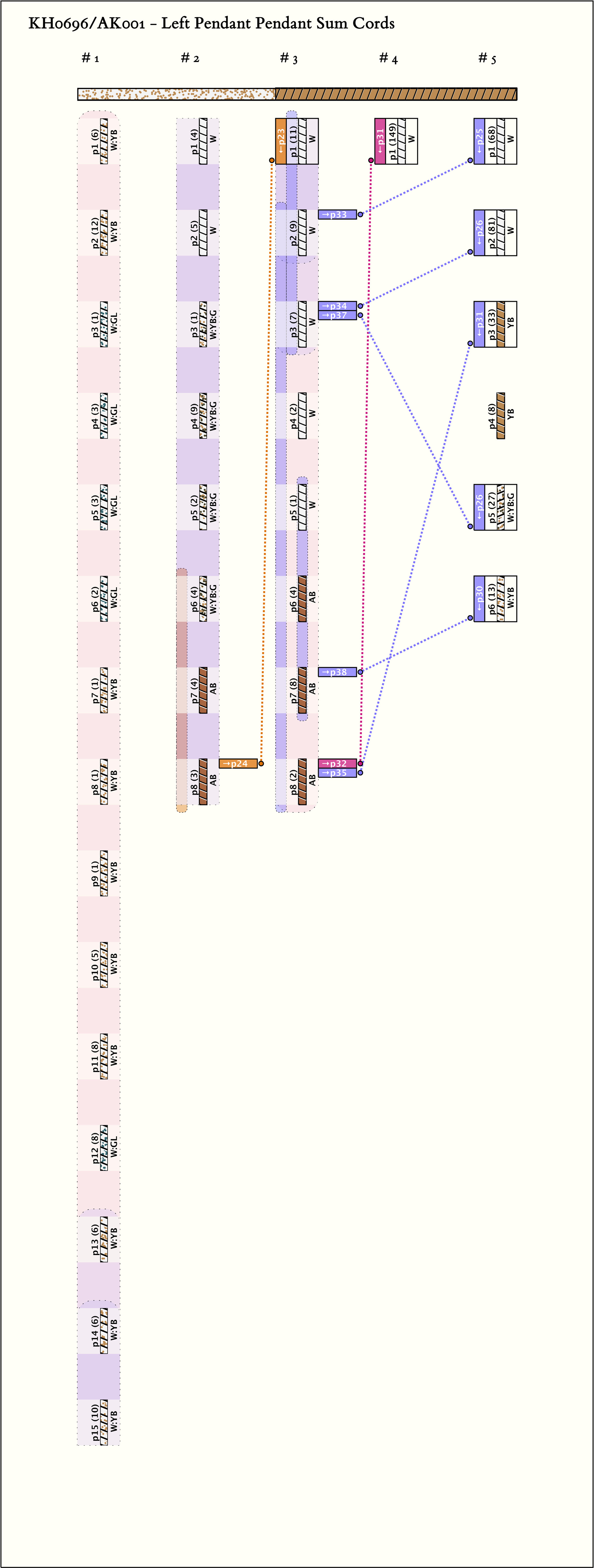
While it is possible to trace the sums in this khipu, it is a bit tedious. And it has several disadventages, including the fact that it requires separate drawings for left and right-handed sums, and that subsidiary cords are not shown.

A sum-map of Left-handed sums shown below, allowed the same information to be revealed in a more efficient manner, albeit with the same disadventages as above.

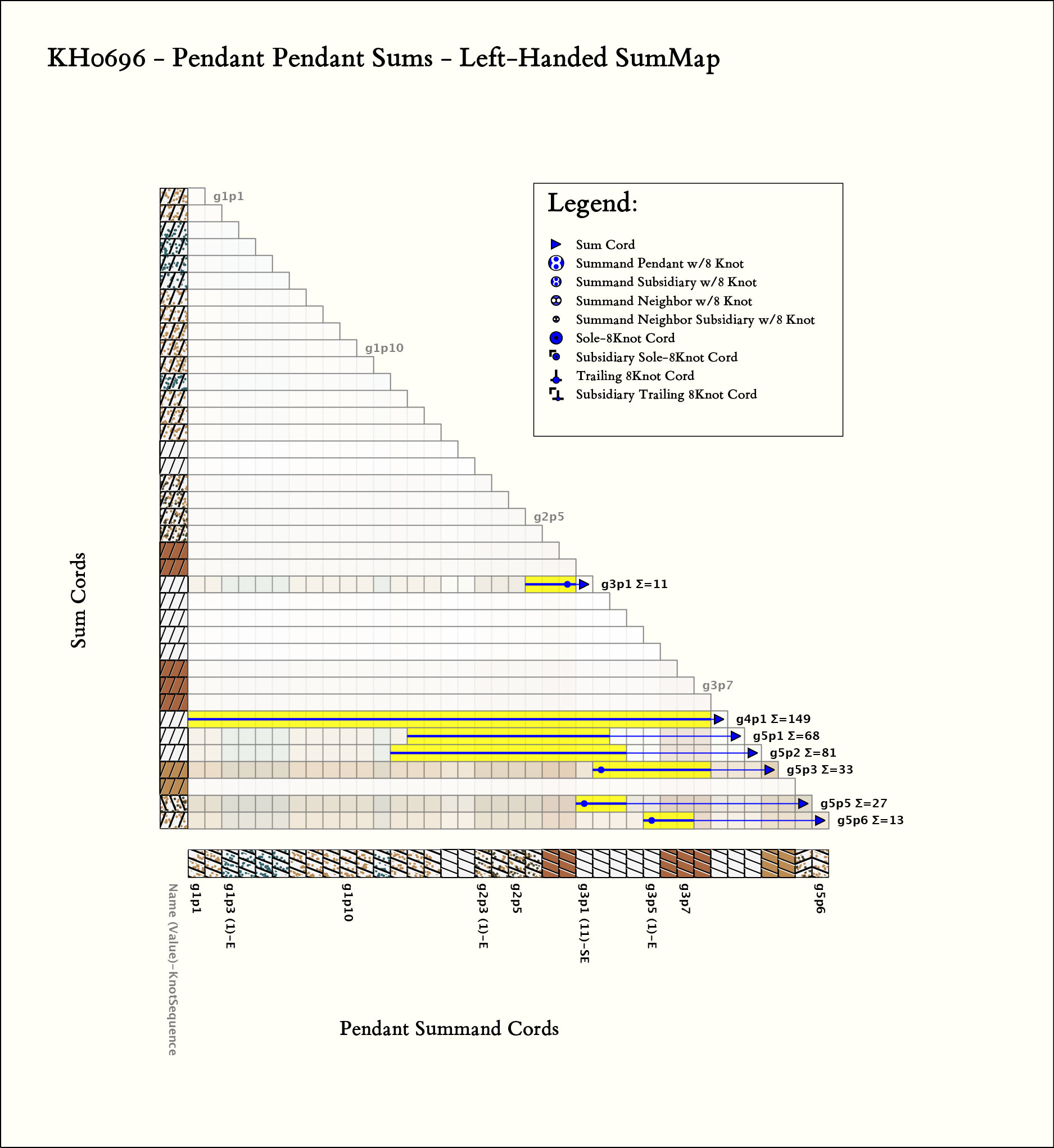
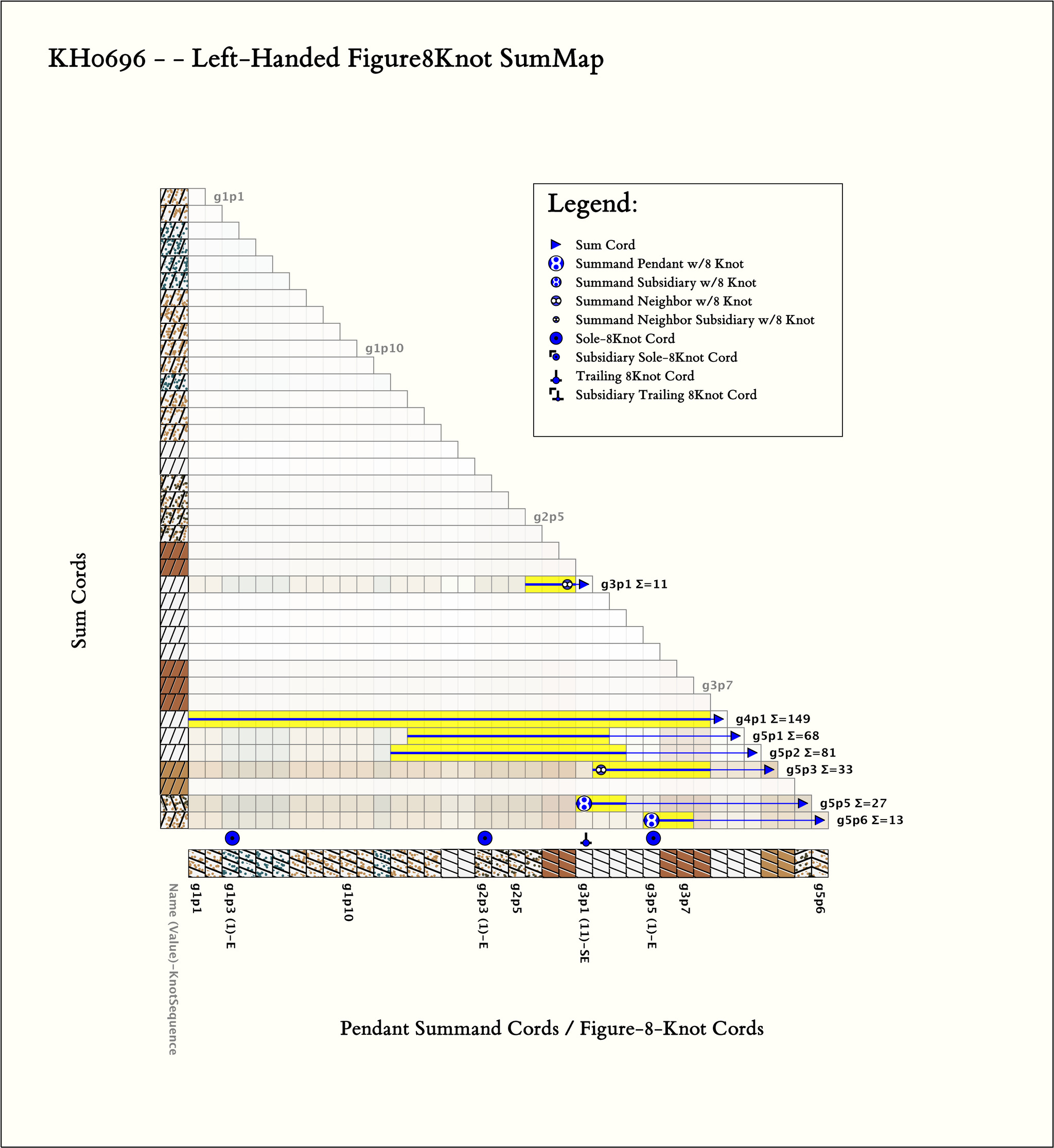
However, this visualization allowed overlaying the sums with additional information, such as the locations of figure-eight knots in sums.

Eventually, it was realized that both left and right-handed sum-maps could be combined to form a single sum-map. This was the breakthrough that allowed equal sums to be discovered.

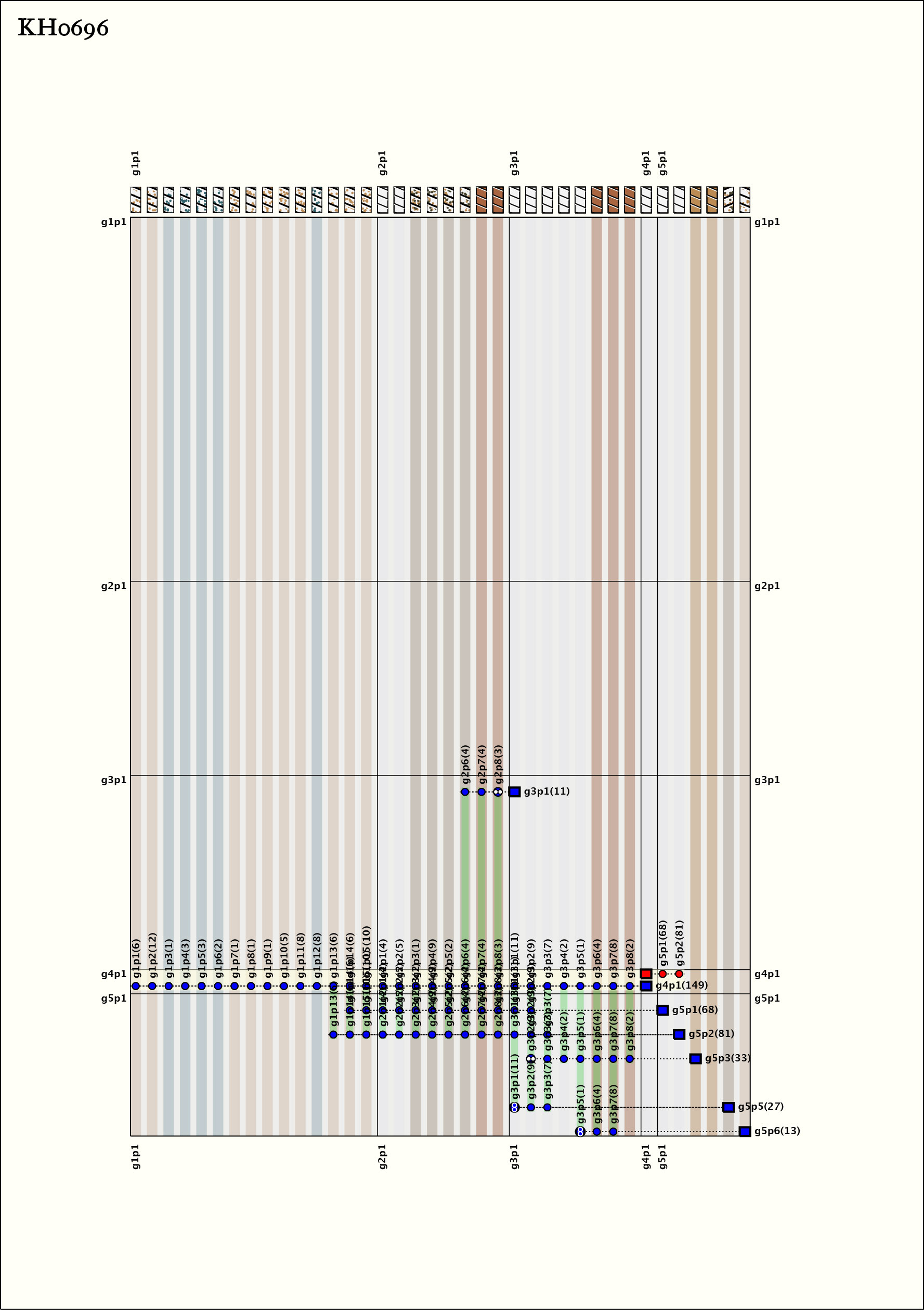
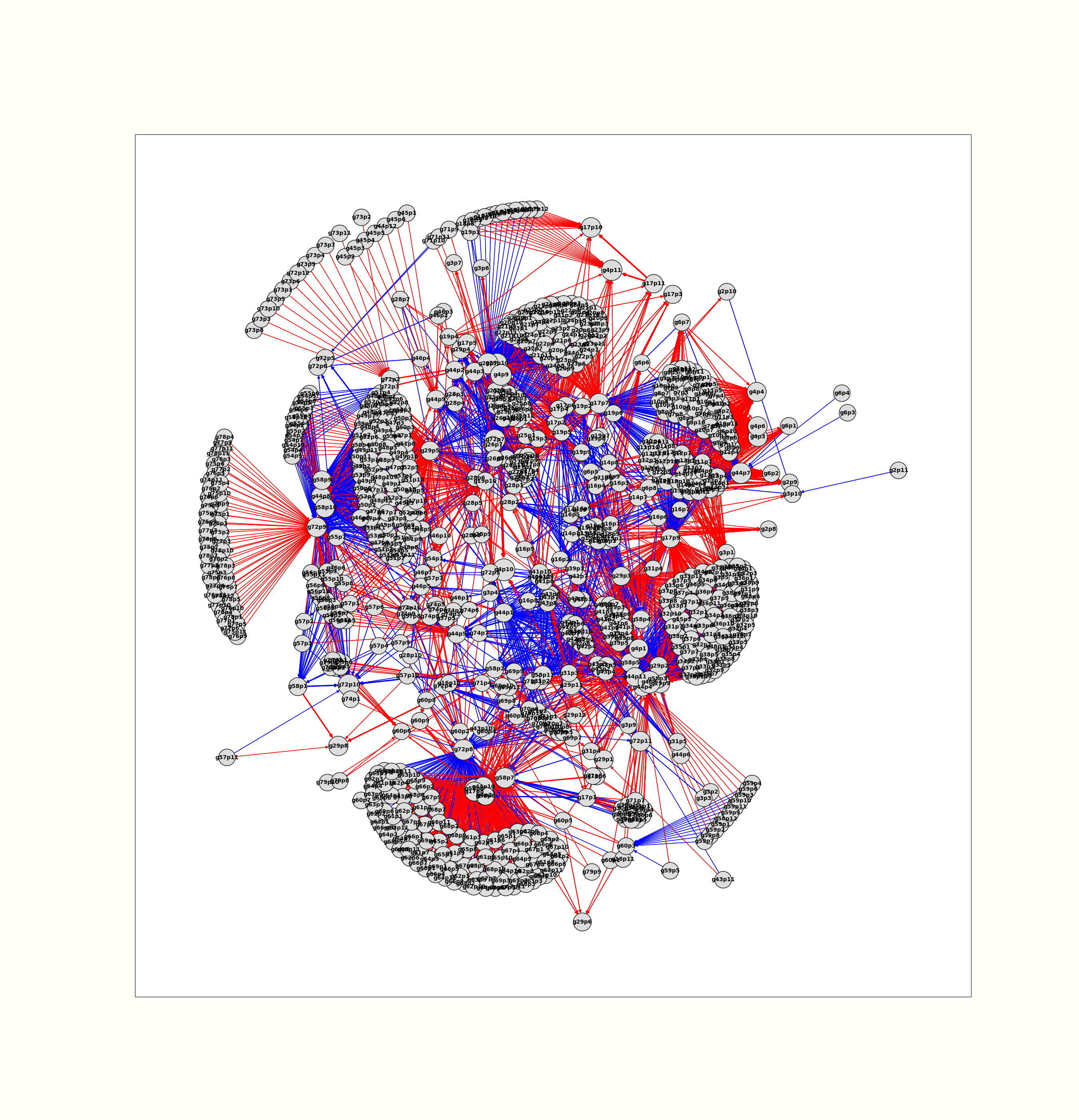
Simultaneously, use of NetworkX graph visualizations, made it easy to reveal the complexity of the patterns in the summations. For examples, look at the sum-graphs of various khipus. in the KFG database. Observe in the sum-graph below, the equal sum g₄p₁ is equal to the sum of the (blue) left-handed sum of all the pendant cords that preceed it, and the (red) right-handed sum of all the pendant cords that follow it, g₅p₁ and g₅p₂. This same pattern is displayed in the combination sum-map above as well.

KH0696 Pendant-Pendant Sum Graph: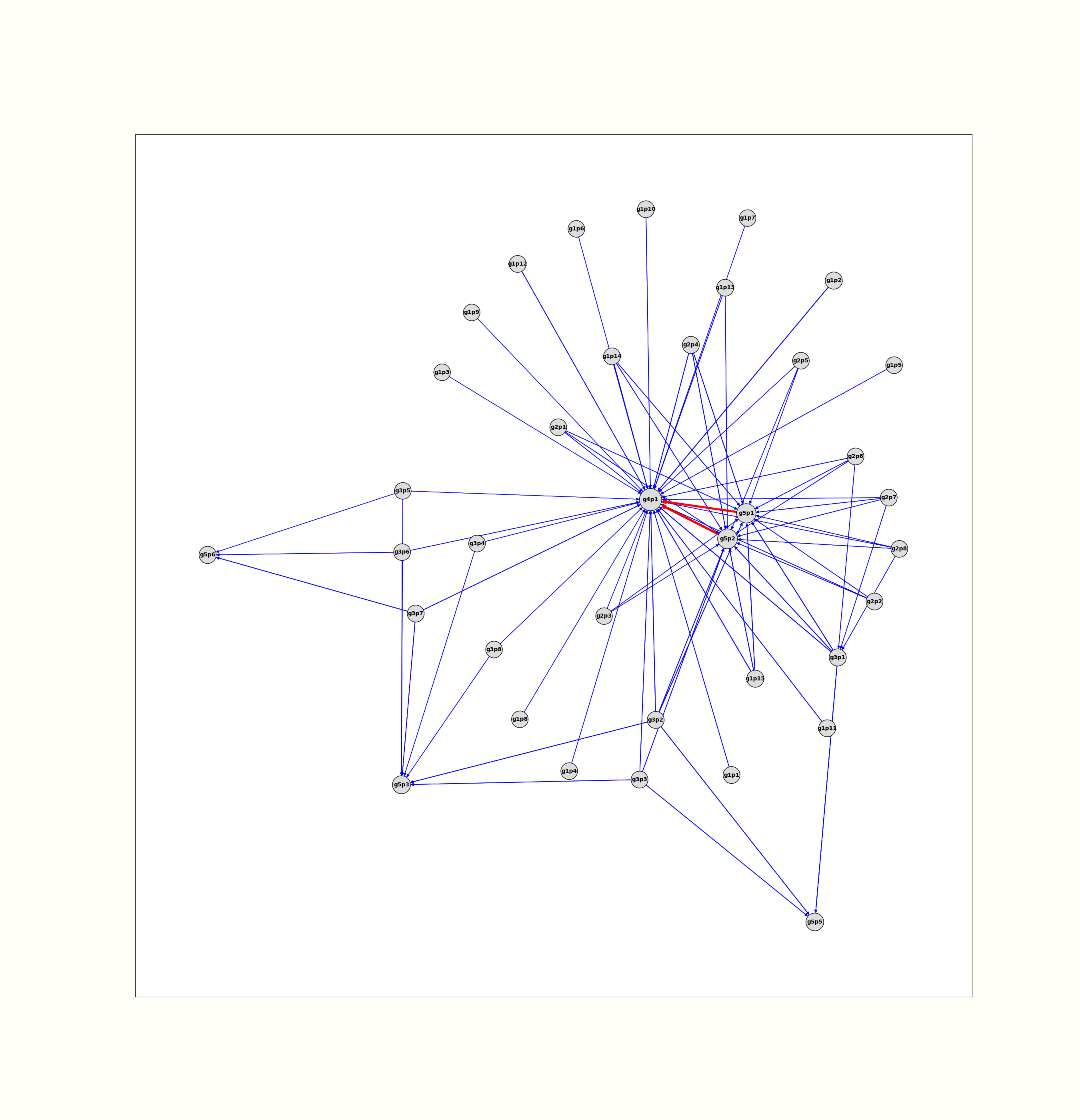

Sum graphs are excellent for visualizing the overall architectural patterns in khipu summations. For example:

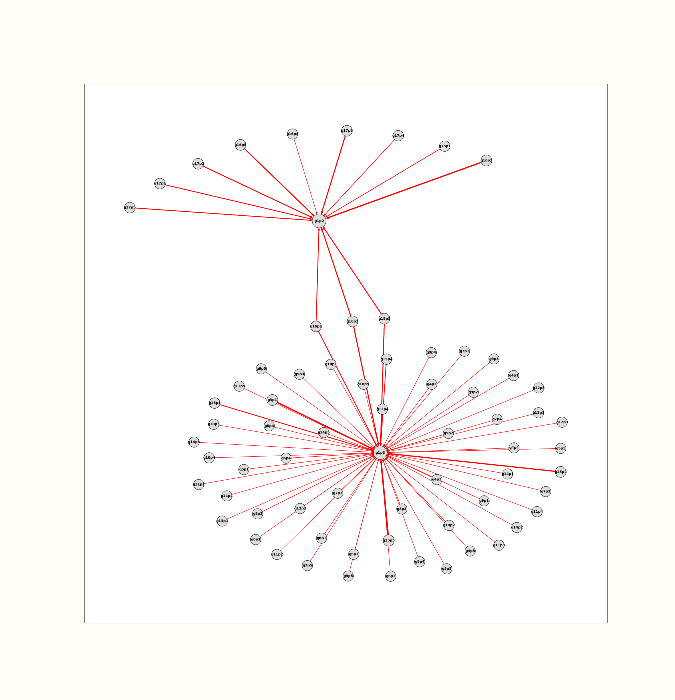
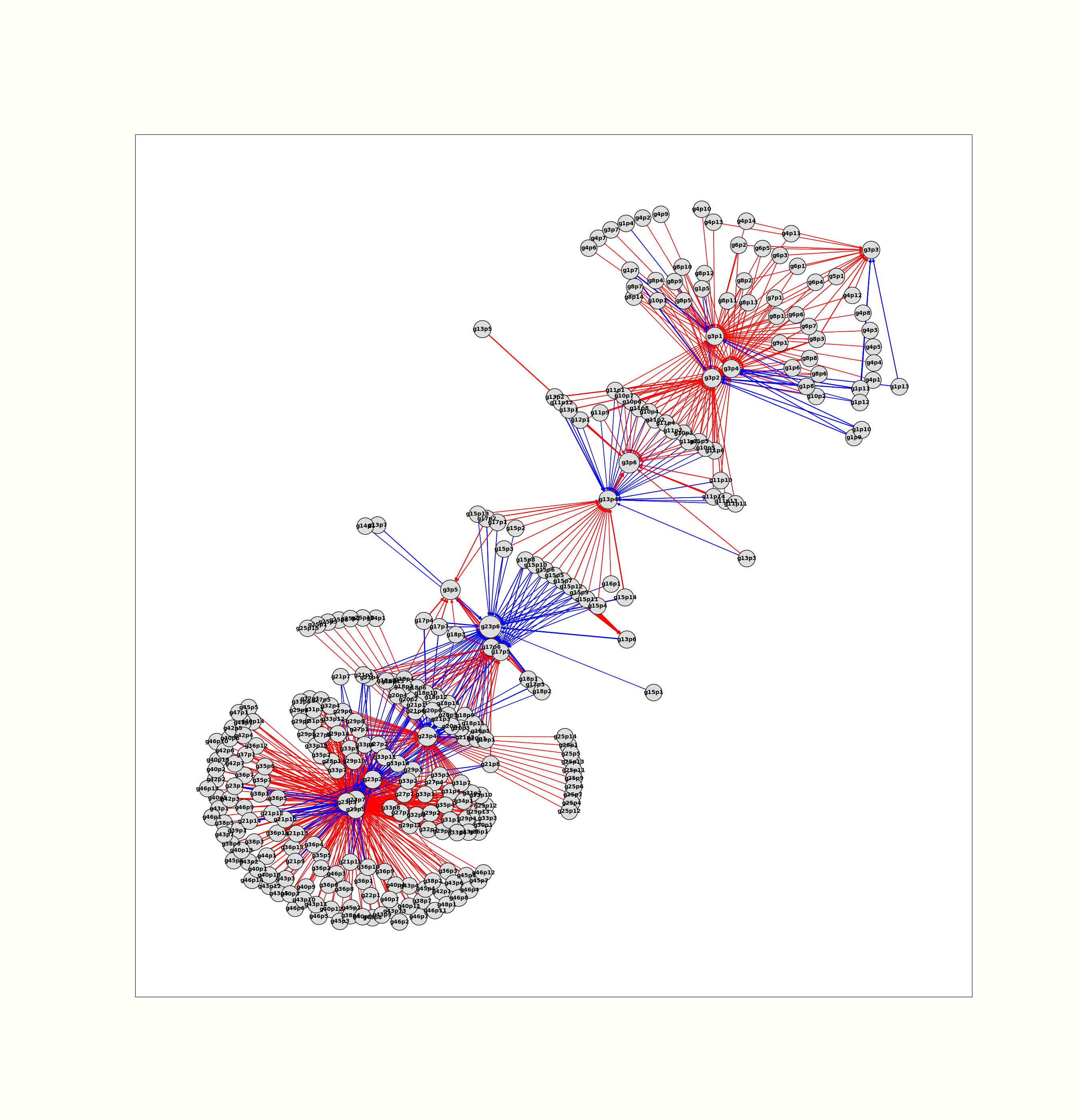
KH0087	KH0068
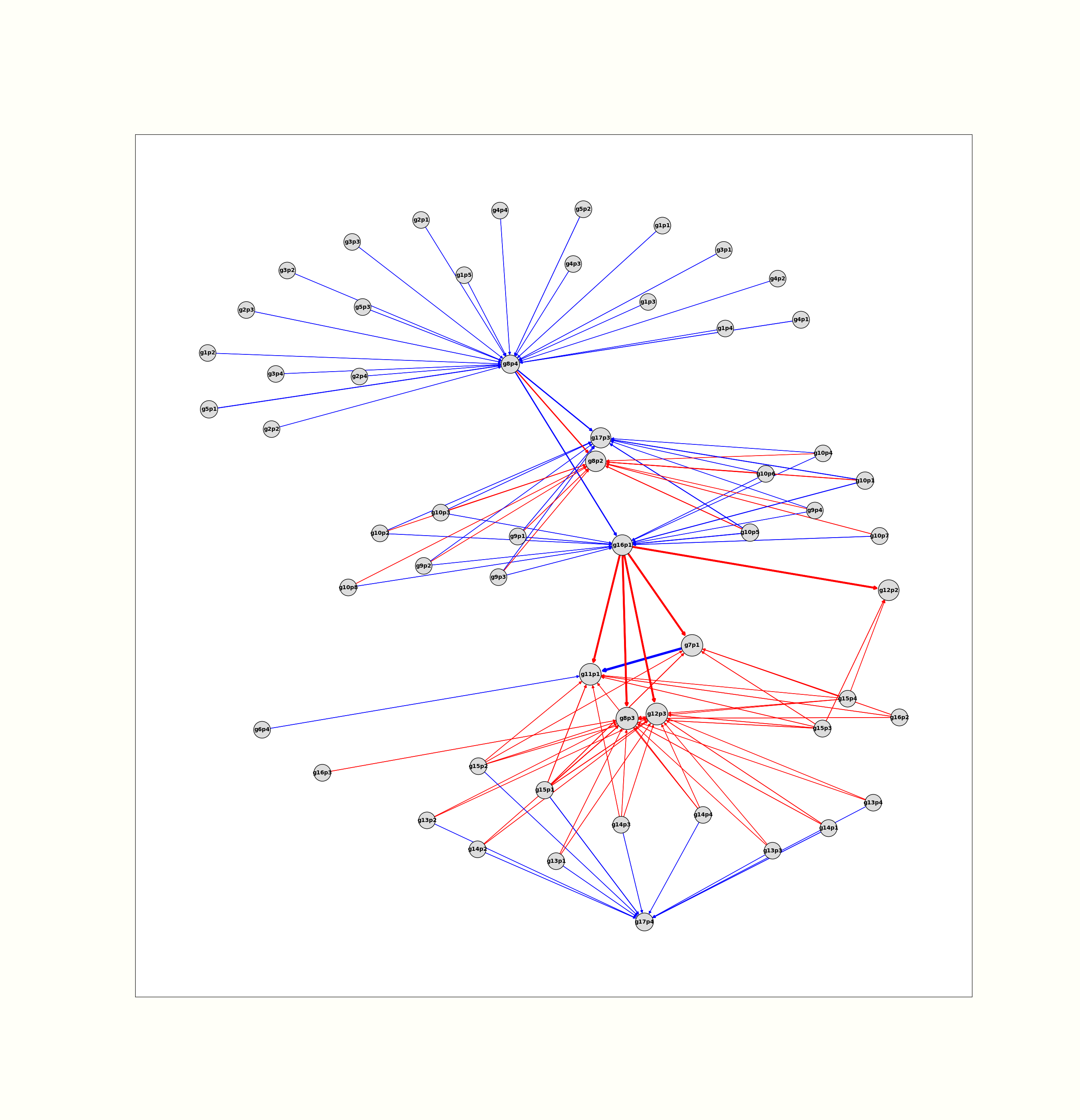
KH0305	KH0468

Finally, it was realized, that the height of a summmap could be considerably reduced. If empty rows in sum-maps were removed, and if a tailored tetris-like space filling algorithm was applied (rows from the top “absorbed” sums from the bottom if there was free space available), then the height of summaps could be considerably reduced, allowing summaps to be drawn directly on the khipu.

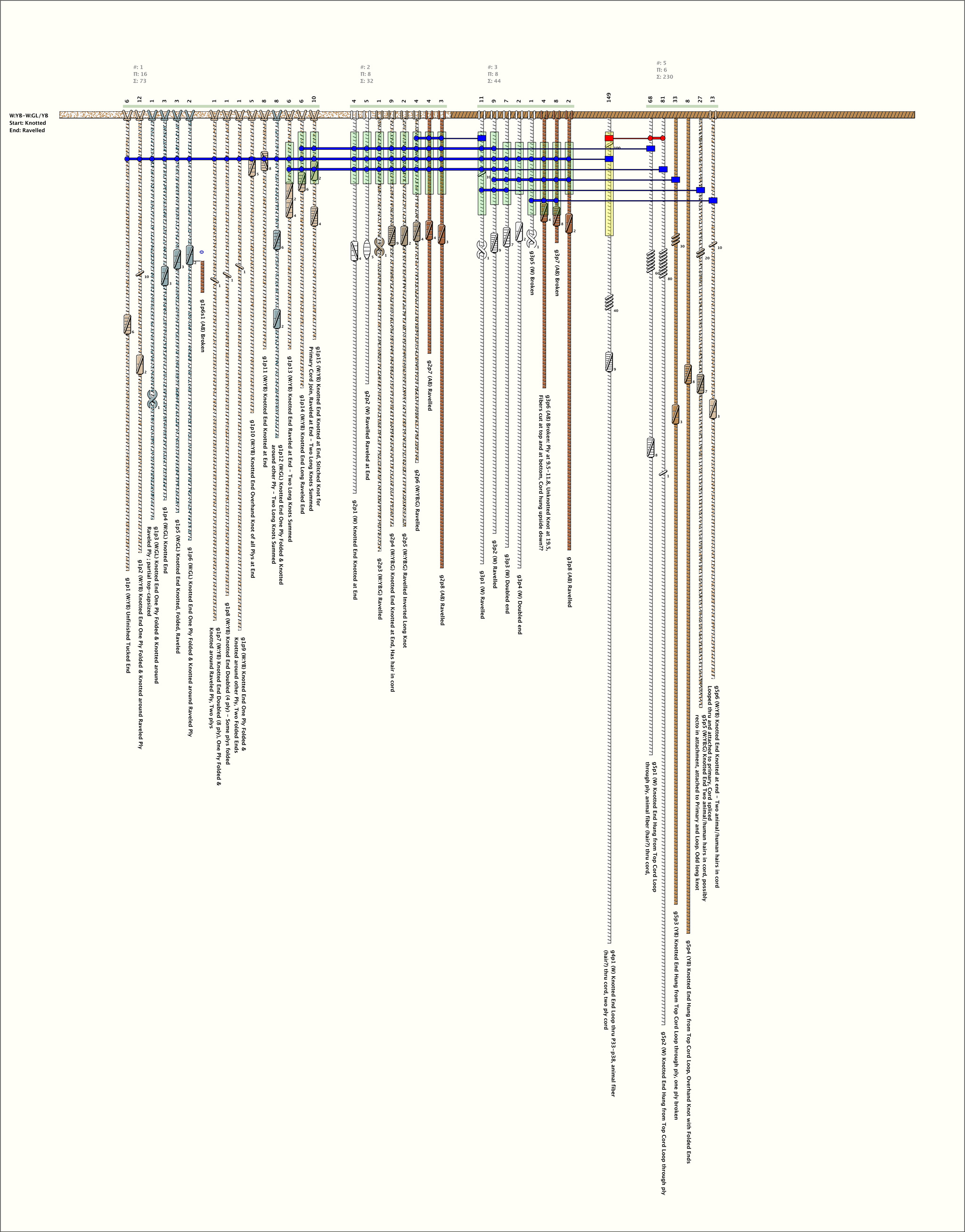
Combining khipus with their sums, allowed the discovery of two important grammatical patterns in khipu summations - Equal Sums, where a Cords value is the sum of both a left-handed and right-handed sums, and Figure-8-Knots, which often mark the boundaries of a summand range.